View and download the notebook here!
Observables#
In the tutorial on params, options, and simulation, we simulated a population of identical individuals: The difference in their behavior was solely due to different random shocks to the reward associated with a choice. In more realistic models, individuals can differ with respect to multiple characteristics, which need to be sampled at the start of the simulation. These characteristics can be:
Experience. Individuals can start with nonzero years of experience for some choice.
Lagged choices. The previous (lagged) choice in the first period can be a subset of all choices in the model.
Observables. An observed characteristic, which does not change over the time-horizon of the model, is not evenly distributed in the population.
Taken together, the assumptions on these characteristics are called the initial conditions of a model. An initial condition is also called a seed value and determines the value of a variable in the first period of a dynamic system.
In this tutorial we will learn how to enrich our baseline Robinson Crusoe economy with observables: The simulated Robinsons will differ with respect to the conditions they experience on the island, which will enter directly the reward for a choice and therefore potentially determine different conditional choice probabilities.
Similarly, in more realistic models, observables such as demographic characteristics or measures of ability need to be controlled for, as they may influence the agents’ behavior.
[1]:
%matplotlib inline

import pandas as pd
import respy as rp
import matplotlib.pyplot as plt
import seaborn as sns
from statsmodels.graphics.mosaicplot import mosaic

# Plot style
sns.set_style("white")
sns.set_context("notebook", font_scale=1.5)
The model: a simple Robinson Crusoe economy, revisited#
We revisit the basic Robinson Crusoe economy. We add one observable characteristic to the baseline model, "Fishing_Grounds": Now Robinson can end up, with a certain probability, on the side of the island which has "poor" or "rich" fishing grounds. Experiencing rich fishing grounds affects the non-pecuniary reward for fishing:
The indicator function \(\unicode{x1D7D9}_{\{condition\}}\) takes value 1 when the condition is true and value 0 otherwise: Therefore, if Robinson finds himself in rich fishing grounds, his total non-pecuniary rewards from fishing will be equal to \(\alpha^f + \zeta^f\).
Specification: params and options#
To introduce observables we need to modify both params and options. The observable needs to be identified by the keyword observable_*_*, while we can use labels to identify its levels (in this case, "rich" and "poor"). Everything after the last underscore is considered to be the level’s label.
First, we load the specifications of the basic model:
[2]:
params, options = rp.get_example_model("robinson_crusoe_basic", with_data=False)
Then, we add three additional rows to params, to specify:
The probability with which Robinson will find himself in rich and in poor fishing grounds;
The value of \(\zeta^f\), which here is set to be positive and constant.
respy allows for complex probability distributions of observables, which may for instance depend on other covariates. However, throughout this tutorial, we will assume that the observables’ probability distributions do not depend on any other information, and we will add them to the model via probability mass function: Each Robinson is randomly assigned to a certain side of the island, according to the float specified under value in the name-level probability.
Note that all probabilities sum to one. If that is not the case, respy will emit a warning and normalize probabilities.
[3]:
params.loc[("observable_fishing_grounds_rich", "probability"), "value"] = 0.5
params.loc[("observable_fishing_grounds_poor", "probability"), "value"] = 0.5
params.loc[("nonpec_fishing", "rich_fishing_grounds"), "value"] = 0.3
[4]:
params
[4]:
| value | ||
|---|---|---|
| category | name | |
| delta | delta | 0.95 |
| wage_fishing | exp_fishing | 0.30 |
| nonpec_fishing | constant | -0.20 |
| nonpec_hammock | constant | 2.00 |
| shocks_sdcorr | sd_fishing | 0.50 |
| sd_hammock | 0.50 | |
| corr_hammock_fishing | 0.00 | |
| observable_fishing_grounds_rich | probability | 0.50 |
| observable_fishing_grounds_poor | probability | 0.50 |
| nonpec_fishing | rich_fishing_grounds | 0.30 |
We also need to overwrite the covariates section of options to include which level of the observable is associated with a higher nonpecuniary reward for fishing:
[5]:
options["covariates"] = {
    "constant": "1",
    "rich_fishing_grounds": "fishing_grounds == 'rich'",
}
Simulation#
We will now sample and simulate 1000 Robinsons, which will differ with respect to their "Fishing_Grounds" value. We will then let the decision rule from the solution of the model guide them for 5 periods, during which their "Fishing_Grounds" value assigned at the start of the simulation cannot change.
[6]:
simulate = rp.get_simulate_func(params, options)
df = simulate(params)
Note that the new characteristic is displayed in a column of the resulting dataset:
[7]:
df.head(20)
[7]:
| Experience_Fishing | Fishing_Grounds | Shock_Reward_Fishing | Meas_Error_Wage_Fishing | Shock_Reward_Hammock | Meas_Error_Wage_Hammock | Choice | Wage | Discount_Rate | Present_Bias | Nonpecuniary_Reward_Fishing | Wage_Fishing | Flow_Utility_Fishing | Value_Function_Fishing | Continuation_Value_Fishing | Nonpecuniary_Reward_Hammock | Wage_Hammock | Flow_Utility_Hammock | Value_Function_Hammock | Continuation_Value_Hammock | ||
|---|---|---|---|---|---|---|---|---|---|---|---|---|---|---|---|---|---|---|---|---|---|
| Identifier | Period | ||||||||||||||||||||
| 0 | 0 | 0 | rich | 1.431303 | 1 | 0.515252 | 1 | fishing | 1.431303 | 0.95 | 1 | 0.1 | 1.431303 | 1.531303 | 10.784925 | 9.740654 | 2 | NaN | 2.515252 | 10.132237 | 8.017878 |
| 1 | 1 | rich | 0.383519 | 1 | 0.529793 | 1 | hammock | NaN | 0.95 | 1 | 0.1 | 0.517697 | 0.617697 | 8.723622 | 8.532553 | 2 | NaN | 2.529793 | 8.988758 | 6.798911 | |
| 2 | 1 | rich | 0.950278 | 1 | -0.189833 | 1 | fishing | 1.282740 | 0.95 | 1 | 0.1 | 1.282740 | 1.382740 | 6.354070 | 5.232979 | 2 | NaN | 1.810167 | 6.025253 | 4.436933 | |
| 3 | 2 | rich | 0.582585 | 1 | -0.585088 | 1 | fishing | 1.061539 | 0.95 | 1 | 0.1 | 1.061539 | 1.161539 | 4.093131 | 3.085887 | 2 | NaN | 1.414912 | 3.822200 | 2.533988 | |
| 4 | 3 | rich | 1.680125 | 1 | -0.108781 | 1 | fishing | 4.132441 | 0.95 | 1 | 0.1 | 4.132441 | 4.232441 | 4.232441 | 0.000000 | 2 | NaN | 1.891219 | 1.891219 | 0.000000 | |
| 1 | 0 | 0 | rich | 1.419559 | 1 | 1.121115 | 1 | fishing | 1.419559 | 0.95 | 1 | 0.1 | 1.419559 | 1.519559 | 10.773181 | 9.740654 | 2 | NaN | 3.121115 | 10.738100 | 8.017878 |
| 1 | 1 | rich | 2.408754 | 1 | 0.133023 | 1 | fishing | 3.251478 | 0.95 | 1 | 0.1 | 3.251478 | 3.351478 | 11.457404 | 8.532553 | 2 | NaN | 2.133023 | 8.591988 | 6.798911 | |
| 2 | 2 | rich | 0.655700 | 1 | 0.650588 | 1 | fishing | 1.194763 | 0.95 | 1 | 0.1 | 1.194763 | 1.294763 | 7.633632 | 6.672494 | 2 | NaN | 2.650588 | 7.621918 | 5.232979 | |
| 3 | 3 | rich | 0.464923 | 1 | -0.308845 | 1 | fishing | 1.143526 | 0.95 | 1 | 0.1 | 1.143526 | 1.243526 | 5.014991 | 3.969963 | 2 | NaN | 1.691155 | 4.622748 | 3.085887 | |
| 4 | 4 | rich | 2.757647 | 1 | -0.133189 | 1 | fishing | 9.155711 | 0.95 | 1 | 0.1 | 9.155711 | 9.255711 | 9.255711 | 0.000000 | 2 | NaN | 1.866811 | 1.866811 | 0.000000 | |
| 2 | 0 | 0 | rich | 1.116904 | 1 | -1.094805 | 1 | fishing | 1.116904 | 0.95 | 1 | 0.1 | 1.116904 | 1.216904 | 10.470526 | 9.740654 | 2 | NaN | 0.905195 | 8.522180 | 8.017878 |
| 1 | 1 | rich | 0.896039 | 1 | 0.452955 | 1 | fishing | 1.209527 | 0.95 | 1 | 0.1 | 1.209527 | 1.309527 | 9.415452 | 8.532553 | 2 | NaN | 2.452955 | 8.911920 | 6.798911 | |
| 2 | 2 | rich | 0.461766 | 1 | 0.762777 | 1 | hammock | NaN | 0.95 | 1 | 0.1 | 0.841392 | 0.941392 | 7.280262 | 6.672494 | 2 | NaN | 2.762777 | 7.734107 | 5.232979 | |
| 3 | 2 | rich | 1.350840 | 1 | 0.571080 | 1 | fishing | 2.461392 | 0.95 | 1 | 0.1 | 2.461392 | 2.561392 | 5.492984 | 3.085887 | 2 | NaN | 2.571080 | 4.978368 | 2.533988 | |
| 4 | 3 | rich | 0.776213 | 1 | 0.410387 | 1 | hammock | NaN | 0.95 | 1 | 0.1 | 1.909176 | 2.009176 | 2.009176 | 0.000000 | 2 | NaN | 2.410387 | 2.410387 | 0.000000 | |
| 3 | 0 | 0 | poor | 1.106631 | 1 | -0.060911 | 1 | fishing | 1.106631 | 0.95 | 1 | -0.2 | 1.106631 | 0.906631 | 9.296601 | 8.831548 | 2 | NaN | 1.939089 | 9.258196 | 7.704322 |
| 1 | 1 | poor | 0.383690 | 1 | -0.377365 | 1 | fishing | 0.517928 | 0.95 | 1 | -0.2 | 0.517928 | 0.317928 | 7.736349 | 7.808865 | 2 | NaN | 1.622635 | 7.695893 | 6.392903 | |
| 2 | 2 | poor | 1.798205 | 1 | -0.600881 | 1 | fishing | 3.276543 | 0.95 | 1 | -0.2 | 3.276543 | 3.076543 | 8.943197 | 6.175425 | 2 | NaN | 1.399119 | 6.045155 | 4.890564 | |
| 3 | 3 | poor | 1.734778 | 1 | -0.466337 | 1 | fishing | 4.266866 | 0.95 | 1 | -0.2 | 4.266866 | 4.066866 | 7.597816 | 3.716790 | 2 | NaN | 1.533663 | 4.281438 | 2.892395 | |
| 4 | 4 | poor | 0.861123 | 1 | -0.354589 | 1 | fishing | 2.859029 | 0.95 | 1 | -0.2 | 2.859029 | 2.659029 | 2.659029 | 0.000000 | 2 | NaN | 1.645411 | 1.645411 | 0.000000 |
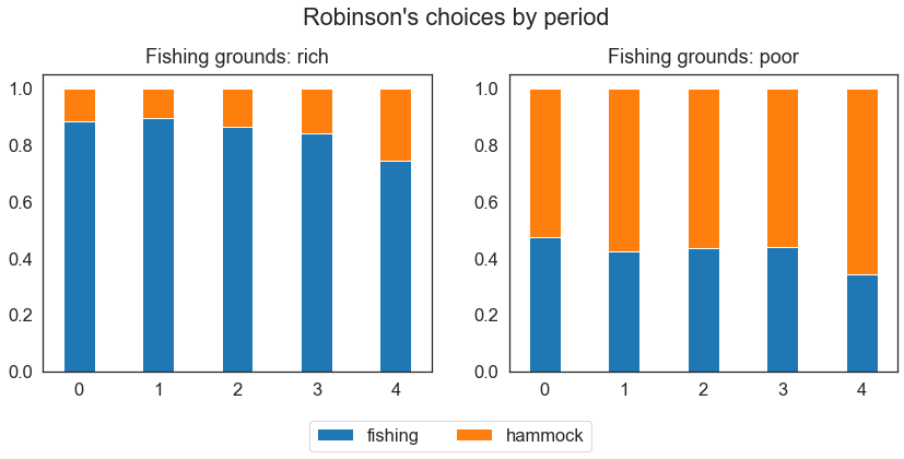
Robinson’s behavior is affected by the observable we introduced: The figure below shows that rich fishing grounds lead to higher engagement in fishing.
[8]:
fig, ax = plt.subplots(1, 2, figsize=(14, 5))

for i, observable in enumerate(["rich", "poor"]):
    df.query("Fishing_Grounds == @observable").groupby("Period").Choice.value_counts(
        normalize=True,
    ).unstack().plot.bar(width=0.4, stacked=True, rot=0, legend=False, ax=ax[i])
    ax[i].set_title("Fishing grounds: " + observable, pad=10)
    ax[i].xaxis.label.set_visible(False)

plt.legend(loc="lower center", bbox_to_anchor=(-0.15, -0.3), ncol=2)
plt.suptitle("Robinson's choices by period", y=1.05)

plt.show()
Multiple observables#
On top of "Fishing_Grounds we add now a second observable, "Cicadas", which also has two evenly distributed levels: "many" or "few". Ending up on a side of the island where many cicadas live affects, this time negatively, the non-pecuniary reward for relaxing on the hammock:
where \(\zeta^h < 0\). The intuition is simple: Robinson finds it less pleasant to spend time on his hammock when he is surrounded by many noisy cicadas.
We again modify params and options to include this new characteristic:
[9]:
params.loc[("observable_cicadas_few", "probability"), "value"] = 0.5
params.loc[("observable_cicadas_many", "probability"), "value"] = 0.5
params.loc[("nonpec_hammock", "many_cicadas"), "value"] = -0.15
[10]:
options["covariates"] = {
    "constant": "1",
    "rich_fishing_grounds": "fishing_grounds == 'rich'",
    "many_cicadas": "cicadas == 'many'",
}
When inspecting a simulated dataset, we can see that the observable "Cicadas" has now its column:
[11]:
simulate = rp.get_simulate_func(params, options)
df_eq = simulate(params)
[12]:
df_eq.head()
[12]:
| Experience_Fishing | Cicadas | Fishing_Grounds | Shock_Reward_Fishing | Meas_Error_Wage_Fishing | Shock_Reward_Hammock | Meas_Error_Wage_Hammock | Choice | Wage | Discount_Rate | ... | Nonpecuniary_Reward_Fishing | Wage_Fishing | Flow_Utility_Fishing | Value_Function_Fishing | Continuation_Value_Fishing | Nonpecuniary_Reward_Hammock | Wage_Hammock | Flow_Utility_Hammock | Value_Function_Hammock | Continuation_Value_Hammock | ||
|---|---|---|---|---|---|---|---|---|---|---|---|---|---|---|---|---|---|---|---|---|---|---|
| Identifier | Period | |||||||||||||||||||||
| 0 | 0 | 0 | many | poor | 1.431303 | 1 | 0.515252 | 1 | fishing | 1.431303 | 0.95 | ... | -0.2 | 1.431303 | 1.231303 | 9.504631 | 8.708766 | 1.85 | NaN | 2.365252 | 9.274431 | 7.272819 |
| 1 | 1 | many | poor | 0.383519 | 1 | 0.529793 | 1 | hammock | NaN | 0.95 | ... | -0.2 | 0.517697 | 0.317697 | 7.664871 | 7.733868 | 1.85 | NaN | 2.379793 | 8.217822 | 6.145294 | |
| 2 | 1 | many | poor | 0.950278 | 1 | -0.189833 | 1 | fishing | 1.282740 | 0.95 | ... | -0.2 | 1.282740 | 1.082740 | 5.605257 | 4.760544 | 1.85 | NaN | 1.660167 | 5.500165 | 4.042104 | |
| 3 | 2 | many | poor | 0.582585 | 1 | -0.585088 | 1 | fishing | 1.061539 | 0.95 | ... | -0.2 | 1.061539 | 0.861539 | 3.555348 | 2.835589 | 1.85 | NaN | 1.264912 | 3.464384 | 2.315234 | |
| 4 | 3 | many | poor | 1.680125 | 1 | -0.108781 | 1 | fishing | 4.132441 | 0.95 | ... | -0.2 | 4.132441 | 3.932441 | 3.932441 | 0.000000 | 1.85 | NaN | 1.741219 | 1.741219 | 0.000000 |
5 rows × 21 columns
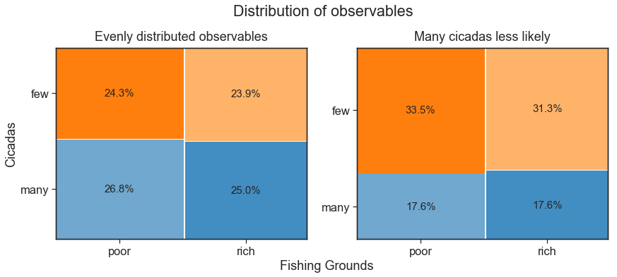
Note that Cicadas and Fishing_Grounds are independent, as we did not specify any additional constraint on their probability distribution.
We can decrease Robinson’s probability of experiencing many cicadas to show how the observables’ distribution changes.
[13]:
params.loc[("observable_cicadas_many", "probability"), "value"] = 0.35
params.loc[("observable_cicadas_few", "probability"), "value"] = 0.65
[14]:
simulate = rp.get_simulate_func(params, options)
df_diff = simulate(params)
[15]:
fig, ax = plt.subplots(1, 2, figsize=(14, 5))

colors = ["#ff7f0e", "#70a8d0", "#ffb369", "#428dc1"]
observables = [
    ("poor", "few"),
    ("poor", "many"),
    ("rich", "few"),
    ("rich", "many"),
]
titles = ["Evenly distributed observables", "Many cicadas less likely"]

for i, df in enumerate([df_eq, df_diff]):

    crosstab = pd.crosstab(df["Fishing_Grounds"], df["Cicadas"], normalize="all")

    properties_dict = {}
    for observable, color in zip(observables, colors):
        properties = {observable: [color, "{:.1%}".format(crosstab.loc[observable])]}
        properties_dict.update(properties)

    mosaic(
        df,
        ["Fishing_Grounds", "Cicadas"],
        ax=ax[i],
        properties=lambda key: {"color": properties_dict[key][0],},
        labelizer=lambda key: properties_dict[key][1],
        gap=0.01,
    )

    ax[i].set_title(titles[i], pad=10)

ax[0].set_xlabel("Fishing Grounds", x=1.08)
ax[0].set_ylabel("Cicadas")

plt.suptitle("Distribution of observables", y=1.05)
plt.show()
Moreover, we can investigate how the within-sample behavior of Robinson changes according to the fishing grounds and the number of cicadas that he experiences:
[16]:
fig, ax = plt.subplots(2, 2, figsize=(14, 10))

ax = ax.flatten()

plt.subplots_adjust(hspace=0.25)

for i, observable in enumerate(observables):
    (
        df_eq.query("Fishing_Grounds == @observable[0] and Cicadas == @observable[1]")
        .groupby("Period")
        .Choice.value_counts(normalize=True)
        .unstack()
        .plot.bar(width=0.4, stacked=True, rot=0, ax=ax[i], legend=False)
    )
    ax[i].xaxis.label.set_visible(False)
    ax[i].set_title(
        observable[0] + " fishing grounds, " + observable[1] + " cicadas", pad=10
    )

plt.legend(loc="right", bbox_to_anchor=(0.3, -0.2), ncol=2)
plt.suptitle("Robinson's choices by period")

plt.show()
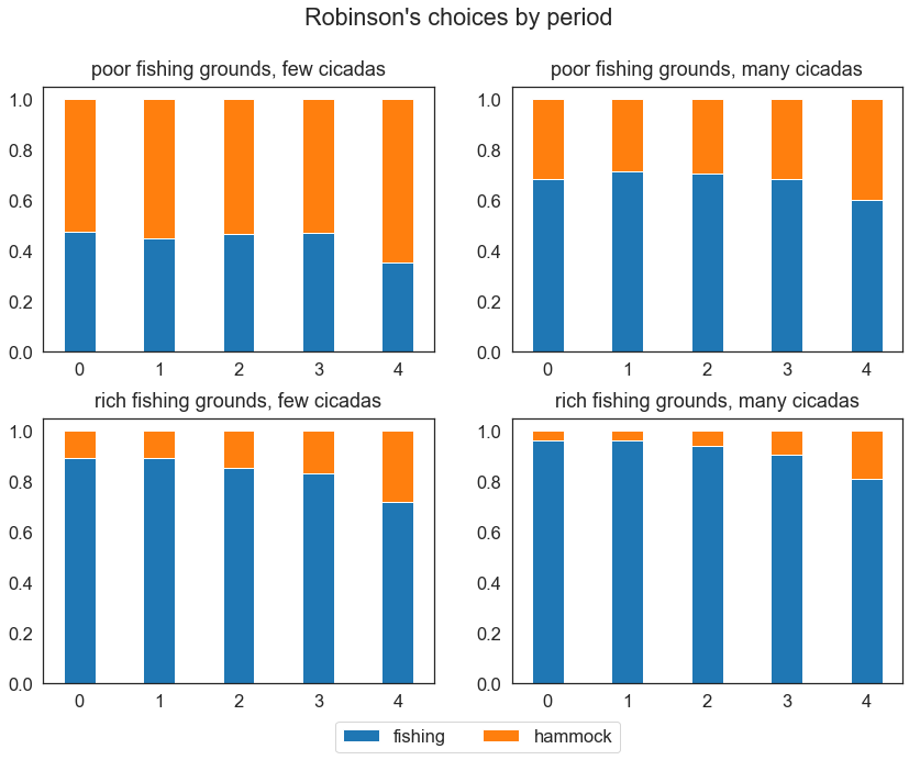
The figure shows that different realizations of observables lead to different incentives for Robinson: His engagement in fishing decreases with poor fishing grounds or few cicadas, while it increases with rich fishing grounds and many cicadas.