View and download the notebook here!

Impatient Robinson

Up to now, we have implicitly assumed Robinson to be forward-looking with respect to his intertemporal preferences, such that he maximizes the expected present value of utility over the remaining lifetime according to

\[U_t(u_t, u_{t+1}, ...) \equiv \sum^{T}_{t=0} {\delta^{t}u_t}\]

where \(\delta \in (0,1]\) is the usual standard discount factor representing time-consistent preferences. With respy you can solve a discrete choice dynamic programming model for a (completely naïve) agent with time-inconsistent preferences just as easily.

We represent time-inconsistency with the popular formulation by O’Donoghue and Rabin (1999): (\(\beta\)-\(\delta\)) preferences, defined as

\[U_t(u_t, u_{t+1}, ...) \equiv u_t + \beta \sum^{T}_{k=t+1} {\delta^{k-t}u_k}\]

where \(\beta \in (0, 1]\) is the present-bias factor that captures time-inconsistent discounting, or impatience; the tendency to prefer activities that are immediately rewarded while procrastinating those that require an immediate cost. If \(\beta = 1\) we are back to the time-consistent case.

In this tutorial, we will see how to model the behavior of an impatient Robinson who is additionally completely naïve with respect to his own time preferences, that is, at each point in time believes he will act time-consistently in future periods.

%matplotlib agg

import io
import yaml

import matplotlib.pyplot as plt
import pandas as pd
import respy as rp
import numpy as np

Specifications

To represent Robinson’s impatience, we just need to add "beta" to the string containing the parameters and specifications of the model. "beta" is by default equal to 1 (time-consistent discounting). Here we set it to 0.4:

params_beta = """
category,name,value
beta,beta, 0.4
delta,delta,0.95
wage_fishing,exp_fishing,0.1
nonpec_fishing,constant,-1
nonpec_hammock,constant,2.5
nonpec_hammock,not_fishing_last_period,-1
shocks_sdcorr,sd_fishing,1
shocks_sdcorr,sd_hammock,1
shocks_sdcorr,corr_hammock_fishing,-0.2
lagged_choice_1_hammock,constant,1
"""

params_beta = pd.read_csv(io.StringIO(params_beta), index_col=["category", "name"])
params_beta

		value
category	name
beta	beta	0.40
delta	delta	0.95
wage_fishing	exp_fishing	0.10
nonpec_fishing	constant	-1.00
nonpec_hammock	constant	2.50
	not_fishing_last_period	-1.00
shocks_sdcorr	sd_fishing	1.00
	sd_hammock	1.00
	corr_hammock_fishing	-0.20
lagged_choice_1_hammock	constant	1.00

In this tutorial, we will compare the behavior of:

1. A time-consistent Robinson ("beta"= 1)

2. An impatient Robinson ("beta" = 0.4)

3. A very impatient Robinson ("beta" = 0.05)

Therefore, we will need two additional sets of params.

# Set of parameters for time-consistent Robinson (as beta is read by default as 1)
params = params_beta.drop(labels="beta", level="category")

# Set of parameters for very impatient Robinson
params_lowbeta = params_beta.copy()
params_lowbeta.loc[("beta", "beta"), "value"] = 0.05

We complement "params" with the options specifications:

options = """n_periods: 10
estimation_draws: 200
estimation_seed: 500
estimation_tau: 0.001
interpolation_points: -1
simulation_agents: 1_000
simulation_seed: 132
solution_draws: 500
solution_seed: 456
covariates:
    constant: "1"
    not_fishing_last_period: "lagged_choice_1 != 'fishing'"
core_state_space_filters:
  # If Robinson has always been fishing, the previous choice cannot be 'hammock'.
  - period > 0 and exp_fishing == period and lagged_choice_1 == 'hammock'
  # If experience in fishing is zero, previous choice cannot be fishing.
  - exp_fishing == 0 and lagged_choice_1 == 'fishing'
"""

options = yaml.safe_load(options)
options

{'n_periods': 10,
 'estimation_draws': 200,
 'estimation_seed': 500,
 'estimation_tau': 0.001,
 'interpolation_points': -1,
 'simulation_agents': 1000,
 'simulation_seed': 132,
 'solution_draws': 500,
 'solution_seed': 456,
 'covariates': {'constant': '1',
  'not_fishing_last_period': "lagged_choice_1 != 'fishing'"},
 'core_state_space_filters': ["period > 0 and exp_fishing == period and lagged_choice_1 == 'hammock'",
  "exp_fishing == 0 and lagged_choice_1 == 'fishing'"]}

Simulation

Basic Model

We start by simulating the basic model for our three Robinsons.

# Simulation for time-consistent Robinson
simulate = rp.get_simulate_func(params, options)
df = simulate(params)

# Simulation for impatient Robinson
simulate = rp.get_simulate_func(params_beta, options)
df_beta = simulate(params_beta)

# Simulation for very impatient Robinson
simulate = rp.get_simulate_func(params_lowbeta, options)
df_lowbeta = simulate(params_lowbeta)

We can then compare their decisions period by period. The grouped stacked bar chart below and all the other visualizations can be easily generated with the Matplotlib library.

fig = plt.figure(figsize=(12, 4))
ax = fig.add_subplot()

x = np.arange(10)

bar_width = 0.25

colors = [["#1f77b4", "#ff7f0e"], ["#428dc1", "#ff9833"], ["#70a8d0", "#ffb369"]]
labels = ["β=1", "β=0.4", "β=0.05"]
positions = [x, x + bar_width * 1.2, x + bar_width * 2.4]

for i, series in enumerate([df, df_beta, df_lowbeta]):
    hammock = series.groupby("Period").Choice.value_counts().unstack().loc[:, "hammock"]
    fishing = series.groupby("Period").Choice.value_counts().unstack().loc[:, "fishing"]
    ax.bar(positions[i], fishing, width=bar_width, color=colors[i][0], label=labels[i])
    ax.bar(
        positions[i],
        hammock,
        width=bar_width,
        bottom=fishing,
        color=colors[i][1],
        label=labels[i],
    )

ax.set_xticks(x + 2 * bar_width / 2)
ax.set_xticklabels(np.arange(10))
ax.set_xlabel("Periods")

handles, _ = ax.get_legend_handles_labels()
handles_positions = [[0, 2, 4], [1, 3, 5]]
bbox_to_anchor = [(1.12, 0.5), (1.12, 0.8)]

for i, title in enumerate(["fishing", "hammock"]):
    legend = plt.legend(
        handles=list(handles[j] for j in handles_positions[i]),
        ncol=1,
        bbox_to_anchor=bbox_to_anchor[i],
        title=title,
        frameon=False,
    )
    plt.gca().add_artist(legend)

fig.suptitle("Robinson's choices", y=0.95);

fig

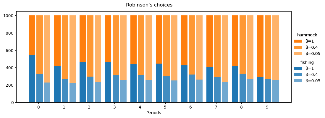
We can see that the impatient Robinsons is less likely to go fishing than the time-consistent Robinson in each period, but even a very impatient Robinson will spend at least two periods fishing.

We can also compare the behavior of the Robinsons for different returns to experience.

# Specification of grid for evaluation
n_points = 15
grid_start = 0
grid_stop = 0.3

grid_points = np.linspace(grid_start, grid_stop, n_points)

mean_max_exp_fishing_by_beta = []
for par in [params, params_beta, params_lowbeta]:
    p = par.copy()
    mean_max_exp_fishing = []
    for value in grid_points:
        p.loc["wage_fishing", "exp_fishing"] = value
        df = simulate(p)
        stat = df.groupby("Identifier")["Experience_Fishing"].max().mean()
        mean_max_exp_fishing.append(stat)
    mean_max_exp_fishing_by_beta.append(mean_max_exp_fishing)

fig, ax = plt.subplots(figsize=(8, 6))
labels = ["β=1", "β=0.4", "β=0.05"]

for mean_max_exp_fishing, label in zip(mean_max_exp_fishing_by_beta, labels):
    plt.plot(grid_points, mean_max_exp_fishing, label=label)

plt.ylim([0, 10])
plt.xlabel("Return to experience")
plt.ylabel("Average final level of experience")

plt.legend();

fig

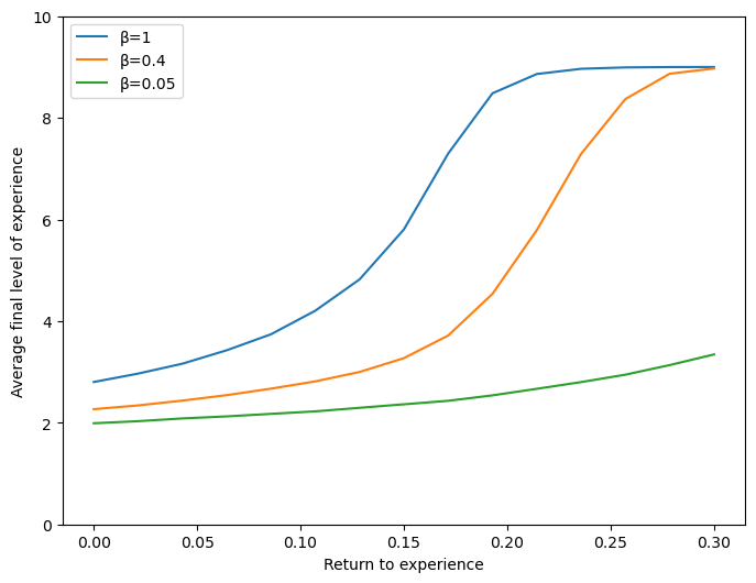
For the same return to experience, time-inconsistent Robinsons attain lower average level of final experience, with the behavior of the very impatient Robinson obviously being the least reactive to an increasing return of experience.

We’ve seen that an impatient agent heavily discounts the stream of utility from future periods. A completely myopic agent, whose preferences are represented by a "delta" equal to 0, does not put any weight on his future utility. We may wonder whether having a very degree of impatience, represented by a very low "beta", may be equivalent to being completely myopic.

# Set of parameters for myopic Robinson
params_myopic = params.copy()
params_myopic.loc[("delta", "delta"), "value"] = 0

# Simulation for myopic Robinson
simulate = rp.get_simulate_func(params_myopic, options)
df_myopic = simulate(params_myopic)

fig, axs = plt.subplots(1, 2, figsize=(12, 4))

df_myopic.groupby("Period").Choice.value_counts().unstack().plot.bar(
    ax=axs[0], stacked=True, rot=0, legend=False, title="Completely myiopic"
)
df_lowbeta.groupby("Period").Choice.value_counts().unstack().plot.bar(
    ax=axs[1], stacked=True, rot=0, title="With present bias (β=0.05)"
)

handles, _ = axs[0].get_legend_handles_labels()
axs[1].get_legend().remove()
fig.legend(handles=handles, loc="lower center", bbox_to_anchor=(0.5, 0), ncol=3)
fig.suptitle("Robinson's choices", fontsize=14, y=1.05)

plt.tight_layout(rect=[0, 0.05, 1, 1])

fig

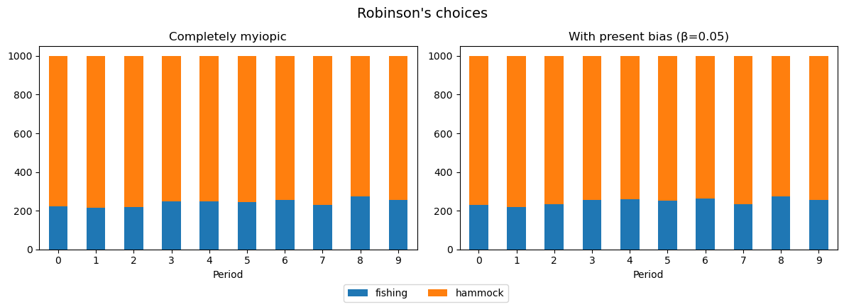
We can see that the behavior of the two Robinsons appear to be identical, despite present-biased Robinson having a long-run discount factor close to 1.

Extended Model

Let’s see what happens in the extended model. Remember that the extended model includes the additional covariate "contemplation_with_friday", a choice available once, starting from the third period, and only if Robinson has been fishing before. Remember that choosing to interact with Friday enters Robinson’s utility negatively, reflecting the effort costs of learning and the food penalty.

This time we compare the behavior of a time-consistent Robinson with that of a time-inconsistent Robinson with "beta" = 0.4. First, we load the model’s options and parameters:

params_ext, options_ext = rp.get_example_model(
    "robinson_crusoe_extended", with_data=False
)

Then, we create another set of parameters for impatient Robinson, which differs from the previous one only in the value of "beta":

index = pd.MultiIndex.from_tuples([("beta", "beta")], names=["category", "name"])
beta = pd.DataFrame(0.4, index=index, columns=["value"])
params_beta_ext = beta.append(params_ext)

Again, we simulate the model for time-consistent and for impatient Robinson:

simulate = rp.get_simulate_func(params_ext, options_ext)
df_ext = simulate(params_ext)

simulate = rp.get_simulate_func(params_beta_ext, options_ext)
df_beta_ext = simulate(params_beta_ext)

We are now ready to compare Robinsons’ choices period by period.

fig, axs = plt.subplots(1, 2, figsize=(12, 4))

df_ext.groupby("Period").Choice.value_counts().unstack().plot.bar(
    ax=axs[0],
    stacked=True,
    rot=0,
    legend=False,
    title="Without present bias",
    color=["C0", "C2", "C1"],
)
df_beta_ext.groupby("Period").Choice.value_counts().unstack().plot.bar(
    ax=axs[1],
    stacked=True,
    rot=0,
    title="With present bias (β=0.4)",
    color=["C0", "C2", "C1"],
)

handles, _ = axs[0].get_legend_handles_labels()
axs[1].get_legend().remove()
fig.legend(handles=handles, loc="lower center", bbox_to_anchor=(0.5, 0), ncol=3)
fig.suptitle("Robinson's choices", fontsize=14, y=1.05)

plt.tight_layout(rect=[0, 0.05, 1, 1])

fig

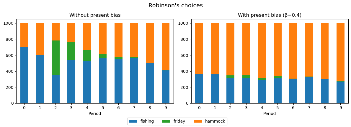
Unsurprisingly, a Robinson who’s a completely naïve, time-incosistent discounter is unlikely to interact with Friday, who would teach him how to fish but affect Robinson’s utility negatively in that period.

References

O’Donoghue, T. and and Rabin, M. (1999). Doing It Now or Later. American Economic Review, 89(1): 103-124.