View and download the notebook here!

Initial Conditions (Experiences, Observables, Lagged Choices)

While working with respy, you often want to simulate the effects of policies in counterfactual environments. At the start of the simulation, you need to sample the characteristics of individuals. You normally want to do at least one of the following points:

• Individuals should start with nonzero years of experience for some choice.

• The previous (lagged) choice in the first period can only be a subset of all choices in the model.

• An observed characteristic is not evenly distributed in the population.

Taken together these assumptions are called the initial conditions of a model. An initial condition is also called a seed value and determines the value of a variable in the first period of a dynamic system.

In the following, we describe how to set the initial condition for each of the the three points for a small Robinson Crusoe Economy. A more thorough presentation of a similar model can be found here.

%matplotlib inline

import io
import pandas as pd
import respy as rp
import matplotlib.pyplot as plt
import seaborn as sns

Experiences

In a nutshell, Robinson can choose between fishing and staying in the hammock every period. He can accumulate experience in fishing which makes him more productive. To describe such a simple model, we write the following parameterization and simulate data with ten periods.

params = """
category,name,value
delta,delta,0.95
wage_fishing,exp_fishing,0.01
nonpec_hammock,constant,1
shocks_sdcorr,sd_fishing,1
shocks_sdcorr,sd_hammock,1
shocks_sdcorr,corr_hammock_fishing,0
"""

options = {
    "n_periods": 10,
    "simulation_agents": 1_000,
    "covariates": {"constant": "1"}
}

params = pd.read_csv(io.StringIO(params), index_col=["category", "name"])
params

		value
category	name
delta	delta	0.95
wage_fishing	exp_fishing	0.01
nonpec_hammock	constant	1.00
shocks_sdcorr	sd_fishing	1.00
	sd_hammock	1.00
	corr_hammock_fishing	0.00

simulate = rp.get_simulate_func(params, options)
df = simulate(params)

fig, axs = plt.subplots(1, 2, figsize=(12.8, 4.8))

(df.groupby("Period").Choice.value_counts(normalize=True).unstack()
 .plot.bar(ax=axs[0], stacked=True, rot=0, title="Choice Probabilities"))
(df.groupby("Period").Experience_Fishing.value_counts(normalize=True).unstack().plot
 .bar(ax=axs[1], stacked=True, rot=0, title="Share of Experience Level per Period", cmap="Reds"))

axs[0].legend(["Fishing", "Hammock"], loc="upper center", bbox_to_anchor=(0.5, -0.15), ncol=2)
axs[1].legend(loc="upper center", bbox_to_anchor=(0.5, -0.15), ncol=5)

plt.show()
plt.close()

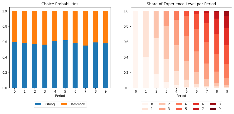
The figure on the left-hand-side shows the choice probabilities for Robinson in each period. On the right-hand-side, one can see the average experience in fishing. By default Robinson starts with zero experience in fishing.

What if Robinson has an equal probability start with zero, one or two periods of experience in fishing? The first way to add more complex initial conditions to the model is via probability mass functions. This type of distributions is handy if the probabilities do not depend on any information. To feed the information to respy use the keyword initial_exp_fishing_* in the category-level of the index. Replace * with the experience level. In the name-level, use probability to signal that the float in value is a probability. The new parameter specification is below.

Note that one probability is set to 0.34 such that all probabilities sum to one. If that is not the case, respy will emit a warning and normalize probabilities.

params = """
category,name,value
delta,delta,0.95
wage_fishing,exp_fishing,0.01
nonpec_hammock,constant,1
shocks_sdcorr,sd_fishing,1
shocks_sdcorr,sd_hammock,1
shocks_sdcorr,corr_hammock_fishing,0
initial_exp_fishing_0,probability,0.33
initial_exp_fishing_1,probability,0.33
initial_exp_fishing_2,probability,0.34
"""

params = pd.read_csv(io.StringIO(params), index_col=["category", "name"])
params

		value
category	name
delta	delta	0.95
wage_fishing	exp_fishing	0.01
nonpec_hammock	constant	1.00
shocks_sdcorr	sd_fishing	1.00
	sd_hammock	1.00
	corr_hammock_fishing	0.00
initial_exp_fishing_0	probability	0.33
initial_exp_fishing_1	probability	0.33
initial_exp_fishing_2	probability	0.34

simulate = rp.get_simulate_func(params, options)
df = simulate(params)

C:\Users\tobia\git\respy\respy\state_space.py:84: UserWarning: Some choices in the model are not admissible all the time. Thus, respy applies a penalty to the utility for these choices which is -400000 by default. For the full solution, the penalty only needs to be larger than all other value functions to be effective. Choose a milder penalty for the interpolation which does not dominate the linear interpolation model.
  "Some choices in the model are not admissible all the time. Thus, respy"

fig, axs = plt.subplots(1, 2, figsize=(12.8, 4.8))

(df.groupby("Period").Choice.value_counts(normalize=True).unstack()
 .plot.bar(ax=axs[0], stacked=True, rot=0, title="Choice Probabilities"))
(df.groupby("Period").Experience_Fishing.value_counts(normalize=True).unstack().plot
 .bar(ax=axs[1], stacked=True, rot=0, title="Share of Experience Level per Period", cmap="Reds"))

axs[0].legend(["Fishing", "Hammock"], loc="upper center", bbox_to_anchor=(0.5, -0.15), ncol=2)
axs[1].legend(loc="upper center", bbox_to_anchor=(0.5, -0.15), ncol=6)

plt.show()
plt.close()

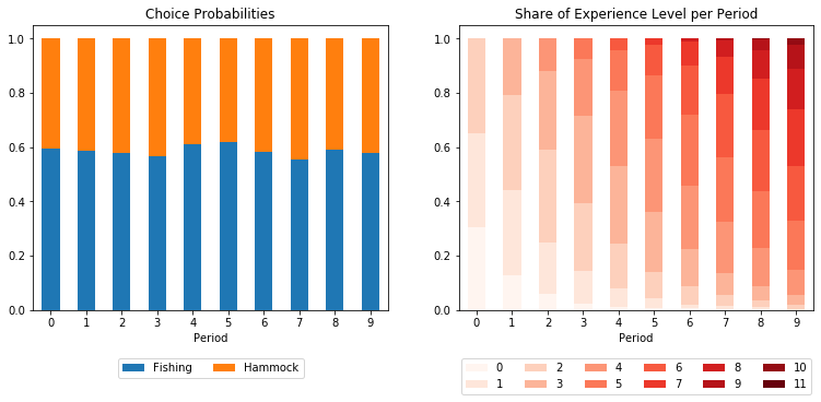
One can clearly see the proportions of experiences in the first period.

Lagged Choices

In the next step, we want to enrich the model with information on the choice in the previous period. Let us assume that Robinson has troubles storing food on a tropical island so that he incurs a penalty if he enjoys his life in the hammock two times in a row. We add the parameter "not_fishing_last_period" to the nonpecuniary reward and add a corresponding covariate to the options.

params = """
category,name,value
delta,delta,0.95
wage_fishing,exp_fishing,0.01
nonpec_hammock,constant,1
nonpec_hammock,not_fishing_last_period,-0.5
shocks_sdcorr,sd_fishing,1
shocks_sdcorr,sd_hammock,1
shocks_sdcorr,corr_hammock_fishing,0
initial_exp_fishing_0,probability,0.33
initial_exp_fishing_1,probability,0.33
initial_exp_fishing_2,probability,0.34
"""

options = {
    "n_periods": 10,
    "simulation_agents": 1_000,
    "covariates": {
        "constant": "1",
        "not_fishing_last_period": "lagged_choice_1 != 'fishing'"
    }
}

params = pd.read_csv(io.StringIO(params), index_col=["category", "name"])
params

		value
category	name
delta	delta	0.95
wage_fishing	exp_fishing	0.01
nonpec_hammock	constant	1.00
	not_fishing_last_period	-0.50
shocks_sdcorr	sd_fishing	1.00
	sd_hammock	1.00
	corr_hammock_fishing	0.00
initial_exp_fishing_0	probability	0.33
initial_exp_fishing_1	probability	0.33
initial_exp_fishing_2	probability	0.34

simulate = rp.get_simulate_func(params, options)
df = simulate(params)

C:\Users\tobia\git\respy\respy\pre_processing\model_processing.py:470: UserWarning: The distribution of initial lagged choices is insufficiently specified in the parameters. Covariates require 1 lagged choices and parameters define 0. Missing lags have equiprobable choices.
  category=UserWarning,
C:\Users\tobia\git\respy\respy\pre_processing\model_processing.py:470: UserWarning: The distribution of initial lagged choices is insufficiently specified in the parameters. Covariates require 1 lagged choices and parameters define 0. Missing lags have equiprobable choices.
  category=UserWarning,

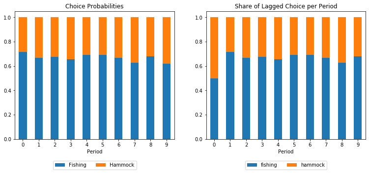
The warning is raised because we forgot to specify what individuals in period 0 have been doing in the previous period. As a default, respy assumes that all choices have the same probability for being the previous choice. Note that, it might lead to inconsistent states where an individual should have accumulated experience in the previous period, but still starts with zero experience.

Below we see the choice probabilities on the left-hand-side and the shares of lagged choices on the right-hand-side. Without further information, respy makes all previous choices in the first period equiprobable.

If we had set the covariate with the lagged choice but not added a parameter using the covariate, respy would have discarded the covariate and created a model without lagged choices.

fig, axs = plt.subplots(1, 2, figsize=(12.8, 4.8))

(df.groupby("Period").Choice.value_counts(normalize=True).unstack()
 .plot.bar(ax=axs[0], stacked=True, rot=0, title="Choice Probabilities"))
(df.groupby("Period").Lagged_Choice_1.value_counts(normalize=True).unstack().plot
 .bar(ax=axs[1], stacked=True, rot=0, title="Share of Lagged Choice per Period"))

axs[0].legend(["Fishing", "Hammock"], loc="upper center", bbox_to_anchor=(0.5, -0.15), ncol=2)
axs[1].legend(loc="upper center", bbox_to_anchor=(0.5, -0.15), ncol=2)

plt.show()
plt.close()

What if we wanted a more complex distribution of lagged choices. Remember that Robinson starts with 0, 1 or 2 periods of experience in fishing. Thus, it is natural to assume that higher experience levels correspond to a higher probability for having fishing as a previous choice.

This kind of distribution is more complex because it involves covariates. A flexible solution is to use a multinomial logit or softmax function to map parameters with covariates to probabilities. This allows to specify very complex distributions, ones which could have been estimated outside the structural model. Here is a short explanation.

For each lag, we have a set of parameters, \(\beta^f\) and \(\beta^h\), and their corresponding covariates, \(x^f\) and \(x^h\). The probability \(p^f\) for one individual having fishing as their first lagged choice is

\[p^f = \frac{e^{x^f \beta^f}}{e^{x^f \beta^f} + e^{x^h \beta^h}}\]

The probability for hammock as the lagged choice is defined analogously.

In the parameters, you can use the lagged_choice_1_fishing keyword to define the parameters for fishing as the first lag. You can also define higher order lags using, for example, lagged_choice_2_*.

Let us assume that with each level of initial experience the probability for choosing fishing the previous period rises from 0.5 over 0.75 to 1. For zero experience in fishing, the resulting probabilities should be one halve for fishing and one halve for hammock. First, we create a covariate which is True if an individual has zero experience in fishing. This covariate is {"zero_exp_fishing": "exp_fishing == 0"}. Then, the parameters for this covariate just have to be equal and can take any value. That is because the softmax function is shift-invariant. The resulting lines in the csv are

lagged_choice_1_fishing,zero_exp_fishing,1
lagged_choice_1_hammock,zero_exp_fishing,1

For one period of experience, the weights are 0.75 for fishing and 0.25 for the hammock. First, define a covariate {"one_exp_fishing": "exp_fishing == 1"}. To get the corresponding softmax coefficients for the probabilities, note that you can rewrite the softmax formula replacing \(x_i\) with 1. Recognize that the sum in the denominator, \(C\), applies to all probabilities and can be discarded. Thus, the coefficients are the logs of the probabilities.

\[\begin{split}\begin{align} p_i &= \frac{e^{x_i \beta_i}}{\sum_j e^{x_j \beta_j}} \\ &= \frac{e^{\beta_i}}{\sum_j e^{\beta_j}} \\ log(p_i) &= \beta_i - \log(\sum_j e^{\beta_j}) \\ &= \beta_i - C \end{align}\end{split}\]

The lines in the parameters for \(log(0.75)\) and \(log(0.25)\) are

lagged_choice_1_fishing,one_exp_fishing,-0.2877
lagged_choice_1_hammock,one_exp_fishing,-1.3863

For two experience in fishing, we have to make sure that fishing receives a probability of one which can be achieved by using a fairly large value such as 6. By default, all missing choices receive a parameter with value -1e300.

The final parameters and options are the following:

params = """
category,name,value
delta,delta,0.95
wage_fishing,exp_fishing,0.01
nonpec_hammock,constant,1
nonpec_hammock,not_fishing_last_period,-0.5
shocks_sdcorr,sd_fishing,1
shocks_sdcorr,sd_hammock,1
shocks_sdcorr,corr_hammock_fishing,0
initial_exp_fishing_0,probability,0.33
initial_exp_fishing_1,probability,0.33
initial_exp_fishing_2,probability,0.34
lagged_choice_1_fishing,zero_exp_fishing,1
lagged_choice_1_hammock,zero_exp_fishing,1
lagged_choice_1_fishing,one_exp_fishing,-0.2877
lagged_choice_1_hammock,one_exp_fishing,-1.3863
lagged_choice_1_fishing,two_exp_fishing,6
"""

options = {
    "n_periods": 10,
    "simulation_agents": 1_000,
    "covariates": {
        "constant": "1",
        "not_fishing_last_period": "lagged_choice_1 != 'fishing'",
        "zero_exp_fishing": "exp_fishing == 0",
        "one_exp_fishing": "exp_fishing == 1",
        "two_exp_fishing": "exp_fishing == 2",
    }
}

params = pd.read_csv(io.StringIO(params), index_col=["category", "name"])
params

		value
category	name
delta	delta	0.9500
wage_fishing	exp_fishing	0.0100
nonpec_hammock	constant	1.0000
	not_fishing_last_period	-0.5000
shocks_sdcorr	sd_fishing	1.0000
	sd_hammock	1.0000
	corr_hammock_fishing	0.0000
initial_exp_fishing_0	probability	0.3300
initial_exp_fishing_1	probability	0.3300
initial_exp_fishing_2	probability	0.3400
lagged_choice_1_fishing	zero_exp_fishing	1.0000
lagged_choice_1_hammock	zero_exp_fishing	1.0000
lagged_choice_1_fishing	one_exp_fishing	-0.2877
lagged_choice_1_hammock	one_exp_fishing	-1.3863
lagged_choice_1_fishing	two_exp_fishing	6.0000

simulate = rp.get_simulate_func(params, options)
df = simulate(params)

C:\Users\tobia\git\respy\respy\state_space.py:84: UserWarning: Some choices in the model are not admissible all the time. Thus, respy applies a penalty to the utility for these choices which is -400000 by default. For the full solution, the penalty only needs to be larger than all other value functions to be effective. Choose a milder penalty for the interpolation which does not dominate the linear interpolation model.
  "Some choices in the model are not admissible all the time. Thus, respy"

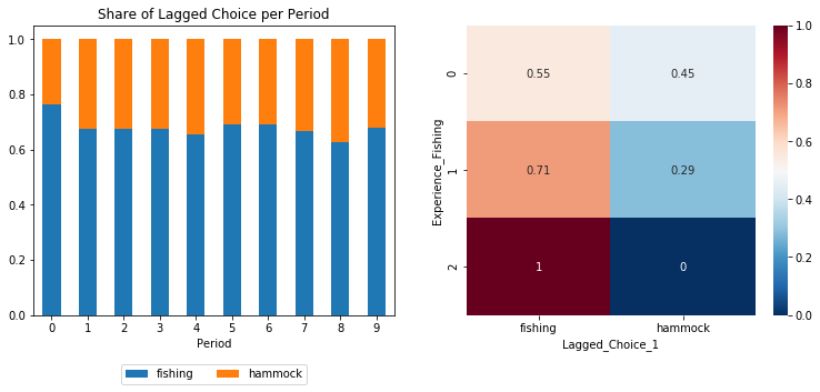
The parameters produce previous choice probabilities on the left-hand-side and the correct conditional probabilities on the right-hand-side. The differences in the probabilities occur due to the low number of simulated individuals.

fig, axs = plt.subplots(1, 2, figsize=(12.8, 4.8))

(df.groupby("Period").Lagged_Choice_1.value_counts(normalize=True).unstack().plot
 .bar(ax=axs[0], stacked=True, rot=0, title="Share of Lagged Choice per Period"))

sns.heatmap((df.query("Period == 0").groupby(["Experience_Fishing"]).Lagged_Choice_1
 .value_counts(normalize="rows").unstack().fillna(0)), ax=axs[1], cmap="RdBu_r", annot=True)

axs[0].legend(loc="upper center", bbox_to_anchor=(0.5, -0.15), ncol=6)

plt.show()
plt.close()

Observables

Now, we have talked enough about experiences and lagged choices. The last section is about observables which are other characteristics such as whether the island has rich fishing grounds or not. We can also express the distribution of observables as probability mass functions or softmax functions.

Note that observables are sampled first before all other characteristics of individuals. After that, experiences and lagged choices in chronological order (highest lag first) follow. Every group itself is sorted alphabetically. Keep this in mind if you want to condition a distribution on other characteristics.

For observables, it is also possible to use labels instead of numbers to identify levels which might be more convenient and intuitive. The evenly distributed levels are "rich" and "poor". The keyword is observable_*_* and everything after the last _ is considered the name of the level.

params = """
category,name,value
delta,delta,0.95
wage_fishing,exp_fishing,0.01
nonpec_fishing,rich_fishing_grounds,0.5
nonpec_hammock,constant,1
nonpec_hammock,not_fishing_last_period,-0.5
shocks_sdcorr,sd_fishing,1
shocks_sdcorr,sd_hammock,1
shocks_sdcorr,corr_hammock_fishing,0
initial_exp_fishing_0,probability,0.33
initial_exp_fishing_1,probability,0.33
initial_exp_fishing_2,probability,0.34
lagged_choice_1_fishing,zero_exp_fishing,1
lagged_choice_1_hammock,zero_exp_fishing,1
lagged_choice_1_fishing,one_exp_fishing,-0.2877
lagged_choice_1_hammock,one_exp_fishing,-1.3863
lagged_choice_1_fishing,two_exp_fishing,6
observable_fishing_grounds_rich,probability,0.5
observable_fishing_grounds_poor,probability,0.5
"""

options = {
    "n_periods": 10,
    "simulation_agents": 10_000,
    "covariates": {
        "constant": "1",
        "not_fishing_last_period": "lagged_choice_1 != 'fishing'",
        "zero_exp_fishing": "exp_fishing == 0",
        "one_exp_fishing": "exp_fishing == 1",
        "two_exp_fishing": "exp_fishing == 2",
        "rich_fishing_grounds": "fishing_grounds == 'rich'",
    }
}

params = pd.read_csv(io.StringIO(params), index_col=["category", "name"])
params

		value
category	name
delta	delta	0.9500
wage_fishing	exp_fishing	0.0100
nonpec_fishing	rich_fishing_grounds	0.5000
nonpec_hammock	constant	1.0000
	not_fishing_last_period	-0.5000
shocks_sdcorr	sd_fishing	1.0000
	sd_hammock	1.0000
	corr_hammock_fishing	0.0000
initial_exp_fishing_0	probability	0.3300
initial_exp_fishing_1	probability	0.3300
initial_exp_fishing_2	probability	0.3400
lagged_choice_1_fishing	zero_exp_fishing	1.0000
lagged_choice_1_hammock	zero_exp_fishing	1.0000
lagged_choice_1_fishing	one_exp_fishing	-0.2877
lagged_choice_1_hammock	one_exp_fishing	-1.3863
lagged_choice_1_fishing	two_exp_fishing	6.0000
observable_fishing_grounds_rich	probability	0.5000
observable_fishing_grounds_poor	probability	0.5000

simulate = rp.get_simulate_func(params, options)
df = simulate(params)

fig, axs = plt.subplots(1, 2, figsize=(12.8, 4.8))

(df.groupby("Fishing_Grounds").Choice.value_counts(normalize=True).unstack().plot
 .bar(ax=axs[0], stacked=True, rot=0, title="Choice Probabilities"))

(df.Fishing_Grounds.value_counts(normalize=True)
 .fillna(0).plot.bar(stacked=True, ax=axs[1], rot=0, title="Observable Distribution"))

axs[0].legend(loc="upper center", bbox_to_anchor=(0.5, -0.15), ncol=2)
axs[1].legend(loc="upper center", bbox_to_anchor=(0.5, -0.15), ncol=2)

plt.show()
plt.close()

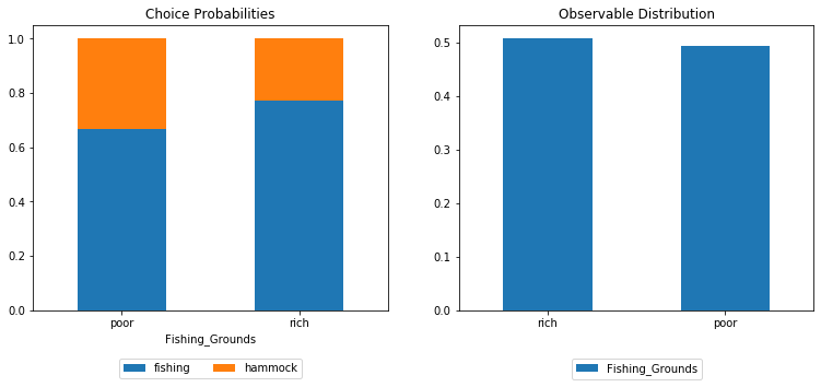
You can see in the figure on the right-hand-side that poor and rich fishing grounds are evenly distributed. The figure on the left-hand-side shows that rich fishing grounds lead to higher engagement in fishing.

Conclusion

We showed …

• how to express different distributions, probability mass functions or softmax functions, in the parameters of a respy model.

• that you can use numbers and labels for discrete levels of observables.

Happy modeling!