View and download the notebook here!

How to Estimate Model Parameters with MSM#

This guide contains an estimation exercise for the use of respy’s method of simulated moments interface with estimagic’s optimization capabilities.

The theoretical basis for the Method of Simulated Moments (MSM) can be found in McFadden (1989). A detailed guide to the MSM interface in respy is linked below. It provides a overview of respy’s MSM functions and outlines how inputs may be specified to construct a criterion function. This guide as a next step showcases a small estimation exercise to estimate parameters with the specified criterion function.

To how-to guide Find out more about Method of Simulated Moments (MSM).

Motivation#

Estimation of structural models is a tedious and complicated task, as it involves the optimization of a usually non-smooth criterion function with respect to a large number of parameters. Optimizers may easily get stuck in local optima for such criterion functions, preventing the finding of a global solution. It is therefore worthwhile to make sure an estimation setup is correctly specified.

The purpose of this exercise is to demonstrate how we can check in a very controlled environment whether an estimation procedure and criterion function are correctly specified for the estimation of a model. This notebook, therefore, is not a guide to estimating a model in general but instead showcases a test of the setup that should precede actual estimation. The exercise also allows us to get a sense of how sensitive the estimation process is to different calibration choices in the optimization like bounds and algorithms, as well as the specification of the criterion function in regards to the choice of weighting matrix, the set of moments, or size of the simulated sample.

In the exercise, we will work with a simulated model which we have complete control of and for which we know the true parameter vector. We will attempt to estimate a misspecified version of the model to perturb the true parameter vector in a controlled fashion and then try to retrieve the parameters for the correct model specification using the perturbed vector as starting values. The exercise thus allows us to test whether the general setup of our optimization problem works and an optimizer is successful in approaching the optimum for a correctly specified model (Eisenhauer et al., 2015; Eisenhauer, 2019).

[1]:

import copy
import numpy as np
import pandas as pd
import matplotlib.pyplot as plt

import respy as rp
from respy.method_of_simulated_moments import _harmonize_input
from estimagic import minimize
from estimagic.logging.create_database import load_database
from estimagic.logging.read_database import read_last_iterations

Setup Estimation#

Note: This guide was created using version 0.0.31 of estimagic and version 2.0.0 of respy. Please note that the guide is not updated regularly so using newer versions of the packages may require adjustments to the code.

Configure MSM Inputs#

To configure the MSM criterion function for estimation, we need to specify a model that will be passed on to the simulator, define moment and replacement functions, derive empirical moments, and specify a weighting matrix. We will use respy’s kw_94_one example model for the exercise, which is based on a model specification from Keane and Wolpin (1994). The following section will outline all the inputs needed to set up the estimation.

Model#

We can generate the model using respy’s get_example_model function. We will treat the parameter vector from this specification as the true parameter vector that we will try to retrieve during estimation. With it comes our observed data that is generated using the true parameters.

[2]:

params, options, data_obs = rp.get_example_model("kw_94_one")

Moment and Replacement Functions#

Aside from the parameters and options that are used to define the model, we need to define functions to compute moments and to replace missing moments in the simulated data during estimation.

[3]:

def calc_choice_frequencies(df):
    """Calculate choice frequencies."""
    return df.groupby("Period").Choice.value_counts(normalize=True).unstack()


def calc_wage_distribution(df):
    """Calculate wage distribution."""
    return df.groupby(["Period"])["Wage"].describe()[["mean", "std"]]


def replace_nans(df):
    """Replace missing values in data."""
    return df.fillna(0)

We save the arguments in dictionaries to later pass on to the criterion function. The function replace_nans can be left as it is because we only use one replacement function for all moments.

[4]:

calc_moments = {
    "Choice Frequencies": calc_choice_frequencies,
    "Wage Distribution": calc_wage_distribution,
}

Empirical Moments#

Now that we have defined the functions needed to compute moments, we can use them to compute the empirical or observed moments for our data. We apply the replacement function to the empirical moments as well.

[5]:

empirical_moments = {
    "Choice Frequencies": replace_nans(calc_choice_frequencies(data_obs)),
    "Wage Distribution": replace_nans(calc_wage_distribution(data_obs)),
}

Weighting Matrix#

Additionally we compute a diagonal variance weighting matrix using a bootstrapping procedure using the function below.

[6]:

def get_weighting_matrix(
    data,
    empirical_moments,
    calc_moments,
    n_bootstrap_samples,
    n_observations_per_sample,
    replace_missing_variances=None,
):
    """ Computes a diagonal weighting matrix for estimation with msm. Weights are the
    inverse bootstrap variances of the observed sample moments."""
    # Seed for reproducibility.
    np.random.seed(123)
    flat_empirical_moments = rp.get_flat_moments(empirical_moments)
    index_base = data.index.get_level_values("Identifier").unique()
    calc_moments = _harmonize_input(calc_moments)
    # Create bootstrapped moments.
    moments_sample = []
    for _ in range(n_bootstrap_samples):
        ids_boot = np.random.choice(
            index_base, n_observations_per_sample, replace=False
        )
        moments_boot = {name: func(data.loc[ids_boot]) for name, func in calc_moments.items()}
        flat_moments_boot = rp.get_flat_moments(moments_boot)
        flat_moments_boot = flat_moments_boot.reindex_like(flat_empirical_moments)
        moments_sample.append(flat_moments_boot)

    # Compute variance for each moment and construct diagonal weighting matrix.
    moments_var = np.array(moments_sample).var(axis=0)

    # The variance of missing moments is nan. Unless a repalcement variance is
    # specified, their inverse variance will be set to 0.
    if replace_missing_variances is None:
        diagonal = moments_var ** (-1)
        diagonal = np.nan_to_num(diagonal, nan=0)
        weighting_matrix = np.diag(diagonal)
    else:
        moments_var = np.nan_to_num(moments_var, nan=replace_missing_variances)
        diagonal = moments_var ** (-1)
        weighting_matrix = np.diag(diagonal)

    # Checks weighting matrix.
    if np.isnan(weighting_matrix).any() or np.isinf(weighting_matrix).any():
        raise ValueError("Weighting matrix contains NaNs or infinite values.")

    return weighting_matrix

[7]:

weighting_matrix = get_weighting_matrix(
    data=data_obs,
    empirical_moments=empirical_moments,
    calc_moments=calc_moments,
    n_bootstrap_samples=300,
    n_observations_per_sample=500,
)

Criterion Function#

Now that we have specified all inputs, we can pass them on to respy’s get_moment_errors_func to generate the criterion function. So far, this guide has just repeated the steps outlined in the general method of simulated moments guide (with the exception of the choice of weighting matrix), now we can move on to the steps required for estimation using the defined criterion function.

[8]:

weighted_sum_squared_errors = rp.get_moment_errors_func(
    params=params,
    options=options,
    calc_moments=calc_moments,
    replace_nans=replace_nans,
    empirical_moments=empirical_moments,
    weighting_matrix=weighting_matrix,
)

Configure Optimization#

In the next step we address the elements that are needed for optimization of the criterion function. These specifications are undertaken specifically for estimation with estimagic. Other optimization packages might require different configurations.

Add Bounds to Parameters#

As a first step we define bounds for our parameter vector that aid the optimizer in estimation. Depending on the model, some parameters may have natural bounds that can be used (i.e. the discount factor ranges between 0 and 1). The choice of bounds is a decisive factor in the success of optimization and may require many adjustments during an actual estimation process when the true parameter values are unknown.

Since this is a simulation exercise, we know the true parameter value and can define our bounds accordingly.

[9]:

def add_params_bounds(params, deviation):
    """ Add upper and lower bounds in parameter vector for optimization."""
    params = params.copy()
    # Compute relative deviation of parameter values as bounds.
    params["lower"] = params["value"] - abs((params["value"] * deviation))
    params["upper"] = params["value"] + abs((params["value"] * deviation))

    # Parameters with value 0 get the absolute deviation as bounds.
    params["upper"] = params["upper"].replace(0, deviation)
    params["lower"] = params["lower"].replace(0, -deviation)

    # Bounds for specififc parameters, shocks do not get bounds.
    params.loc[("delta", "delta"), ("lower", "upper")] = (0, 1)
    params.loc["shocks_sdcorr", ("lower", "upper")] = (-(np.inf), np.inf)

    return params

Below, we select bounds that constitute a 5% deviation from the true values (or an absolute deviation of 0.05 for parameters that are 0 at the true value. Note that the columns should be named lower and upper so estimagic can recognize them as bounds.

[10]:

params = add_params_bounds(params, 0.05)

[11]:

params

[11]:

		value	comment	lower	upper
category	name
delta	delta	0.9500	discount factor	0.000000e+00	1.000000e+00
wage_a	constant	9.2100	log of rental price	8.749500e+00	9.670500e+00
	exp_edu	0.0380	return to an additional year of schooling	3.610000e-02	3.990000e-02
	exp_a	0.0330	return to same sector experience	3.135000e-02	3.465000e-02
	exp_a_square	-0.0005	return to same sector, quadratic experience	-5.250000e-04	-4.750000e-04
	exp_b	0.0000	return to other sector experience	-5.000000e-02	5.000000e-02
	exp_b_square	0.0000	return to other sector, quadratic experience	-5.000000e-02	5.000000e-02
wage_b	constant	8.4800	log of rental price	8.056000e+00	8.904000e+00
	exp_edu	0.0700	return to an additional year of schooling	6.650000e-02	7.350000e-02
	exp_b	0.0670	return to same sector experience	6.365000e-02	7.035000e-02
	exp_b_square	-0.0010	return to same sector, quadratic experience	-1.050000e-03	-9.500000e-04
	exp_a	0.0220	return to other sector experience	2.090000e-02	2.310000e-02
	exp_a_square	-0.0005	return to other sector, quadratic experience	-5.250000e-04	-4.750000e-04
nonpec_edu	constant	0.0000	constant reward for choosing education	-5.000000e-02	5.000000e-02
	at_least_twelve_exp_edu	0.0000	reward for going to college (tuition, etc.)	-5.000000e-02	5.000000e-02
	not_edu_last_period	-4000.0000	reward for going back to school	-4.200000e+03	-3.800000e+03
nonpec_home	constant	17750.0000	constant reward of non-market alternative	1.686250e+04	1.863750e+04
shocks_sdcorr	sd_a	0.2000	Element 1,1 of standard-deviation/correlation ...	-inf	inf
	sd_b	0.2500	Element 2,2 of standard-deviation/correlation ...	-inf	inf
	sd_edu	1500.0000	Element 3,3 of standard-deviation/correlation ...	-inf	inf
	sd_home	1500.0000	Element 4,4 of standard-deviation/correlation ...	-inf	inf
	corr_b_a	0.0000	Element 2,1 of standard-deviation/correlation ...	-inf	inf
	corr_edu_a	0.0000	Element 3,1 of standard-deviation/correlation ...	-inf	inf
	corr_edu_b	0.0000	Element 3,2 of standard-deviation/correlation ...	-inf	inf
	corr_home_a	0.0000	Element 4,1 of standard-deviation/correlation ...	-inf	inf
	corr_home_b	0.0000	Element 4,2 of standard-deviation/correlation ...	-inf	inf
	corr_home_edu	0.0000	Element 4,3 of standard-deviation/correlation ...	-inf	inf
lagged_choice_1_edu	probability	1.0000	Probability that the first lagged choice is ed...	9.500000e-01	1.050000e+00
initial_exp_edu_10	probability	1.0000	Probability that the initial level of educatio...	9.500000e-01	1.050000e+00
maximum_exp	edu	20.0000	Maximum level of experience for education (opt...	1.900000e+01	2.100000e+01
inadmissibility_penalty	inadmissibility_penalty	-400000.0000	Penalty to non-pecuniary reward for invalid ch...	-4.200000e+05	-3.800000e+05

Select Algorithm and Constraints#

There are additional arguments we need to pass on to the optimizer like the optimization algorithm and constraints. We can get the constraints for the selected model from respy using the function get_parameter_constraints. We collect the elements in a dictionary that can be passed on to the optimizer.

[12]:

optim_config = {
    "algorithm": "nlopt_bobyqa",
    "constraints": rp.get_parameter_constraints("kw_94_one"),
}

Estimation Exercise#

Finally, we can perform the estimation exercise. The target of this exercise is to test whether an optimizer manages to retrieve the true parameter vector (approximately) after we have induced it to distance itself from the true values. To generate starting values for the estimation that differ from the true vector, we misspecify the model by fixing the discount factor to 0, thus rendering agents myopic in our model. We then attempt to estimate the parameters for the misspecified model but will fail to retrieve them as the discount factor is fixed to zero. Within the bounds chosen above, the estimated values for the free parameters will thus diverge from the true ones we started with.

In the next step, delta is fixed back to the correct value and the resulting parameter vector from the last step is used as the starting vector for the new estimation. During this estimation, the simulated moments should converge back to the observed ones.

In short, the exercise comprises the following steps.

Begin with the true parameter vector, set delta to 0, and fix it in the constraints, thereby misspecifying the model.
Estimate the free parameters for the misspecified model for a selected number of maximum evaluations of the criterion function.
Using the resulting parameter vector from (2) as start values, set delta back to its true value.
Estimate the parameters using the vector from (3) as start values.

[13]:

def delta_exercise(
    params_true, criterion, optim_config, eval_away, eval_back,
):
    """
    Exercise to test estimation setup. Model is estimated twice: once for a
    misspecified parameter vector and then again for a correct specification.
    """
    configuration = copy.deepcopy(optim_config)

    # 1. Fix delta to 0 in the parameter vector.
    start_away = params_true.copy()
    start_away.loc["delta", "value"] = 0

    configuration["constraints"] += [{"loc": "delta", "type": "fixed"}]
    configuration["algo_options"] = {"maxeval": eval_away}

    # 2. Run optimization with misspecified model.
    rslt_away = minimize(
        criterion, params=start_away, logging="logging_away.db", **configuration
    )

    # 3. Set delta back to true value.
    start_back = rslt_away[1][["value", "upper", "lower"]].copy()
    start_back.loc[("delta", "delta"), "value"] = params_true.loc[
        ("delta", "delta"), "value"
    ]
    configuration["algo_options"] = {"maxeval": eval_back}

    # 4. Estimate again.
    rslt_back = minimize(
        criterion, params=start_back, logging="logging_back.db", **configuration
    )

    # 5. Save results.
    params_dict = {
        "(1) Start value with delta=0": start_away,
        "(2) Result with delta=0": rslt_away[1],
        "(3) New starting vector correct delta": start_back,
        "(4) Final result": rslt_back[1],
    }

    return params_dict

We use the function above to perform the exercise. The function returns a dictionary with the parameter vector at different steps in the exercise. Additionally, the optimizations are monitored in the databases logging_away.db and logging_back.db for step (2) and step (4) respectively.

[14]:

params_dict = delta_exercise(
    params_true=params,
    criterion=weighted_sum_squared_errors,
    optim_config=optim_config,
    eval_away=200,
    eval_back=200,
)

Results#

To evaluate the results of our exercise, there are multiple metrics we should assess. The first and easiest one is the criterion value itself. Since the objective of the optimization is to minimize the the weighted squared difference between empirical and simulated moments, the criterion value should decrease during optimization. If this is not the case, we have an immediate indicator that we made a mistake in our configuration.

Criterion Value#

The criterion values during our exercise decrease for both optimizations. Interestingly, the value is actually lower at step (2) for the misspecified model that at step (4) for the correctly specified model. Only looking at the criterion value thus might lead to wrong conclusions about the parameter estimates. We therefore in the next section turn to the model moments implied by our estimates.

[15]:

for key in params_dict:
    print(f"Criterion value for {key}: ", round(weighted_sum_squared_errors(params_dict[key]), 1))

Criterion value for (1) Start value with delta=0:  766160.6
Criterion value for (2) Result with delta=0:  58334.3
Criterion value for (3) New starting vector correct delta:  297888.4
Criterion value for (4) Final result:  85052.4

Moments#

After inspecting the criterion values, we are interested in how well the estimated parameters manage to fit the moments we selected for estimation, especially the choices of individuals in each period. We thus compute the moments for all parameter vectors that were saved to params_dict. The function get_moment_errors_func can generate a criterion function that returns simulated moments in addition to the function value. We thus generate a new criterion function with the argument return_simulated_moments set to True.

[16]:

get_simulated_moments = rp.get_moment_errors_func(
    params=params,
    options=options,
    calc_moments=calc_moments,
    replace_nans=replace_nans,
    empirical_moments=empirical_moments,
    weighting_matrix=weighting_matrix,
    return_simulated_moments=True,
)

Now we can use the function to compute and plot the simulated moments at each step in the exercise.

[17]:

def plot_moments(params_dict, criterion, empirical_moments, moment_set, ymin, ymax):
    """Plot moments generated by parameter dictionary against empirical moments."""
    fig, axes = plt.subplots(3, 2, figsize=(12, 10))
    axes = axes.ravel()
    for i, key in enumerate(params_dict):
        _, moments = get_simulated_moments(params_dict[key])
        moments[moment_set].plot(ax=axes[i], title=key, ylim=[ymin, ymax])
        plt.tight_layout()

    empirical_moments[moment_set].plot(ax=axes[4], title="Observed", ylim=[ymin, ymax])
    fig.delaxes(axes[5])

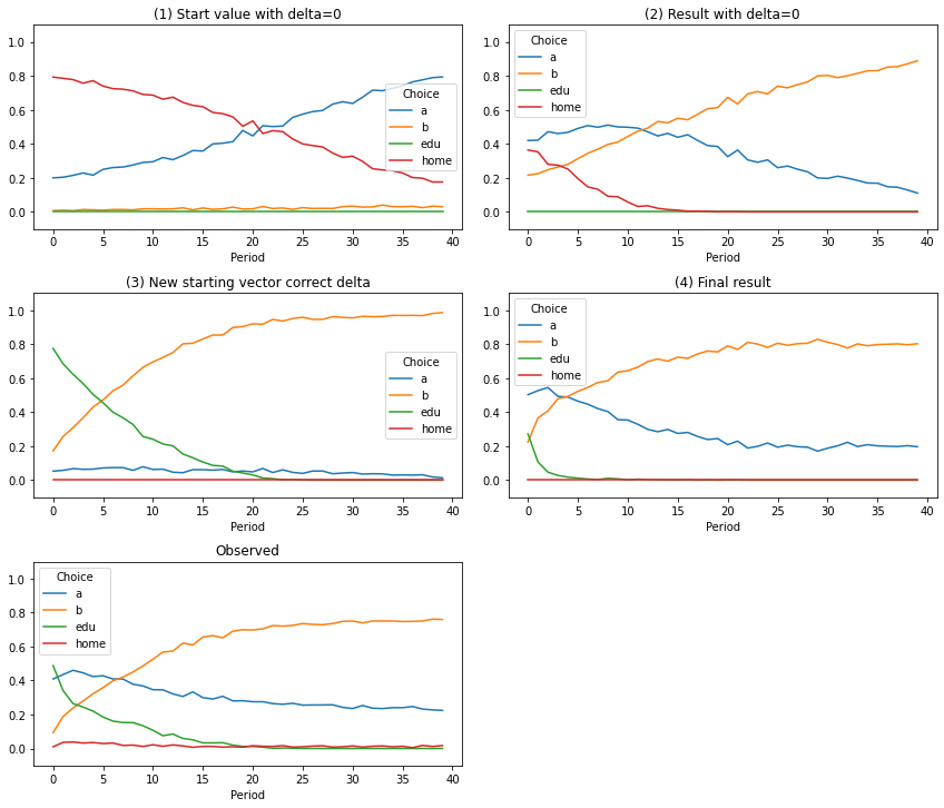
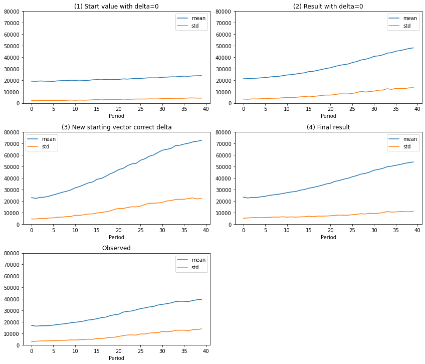
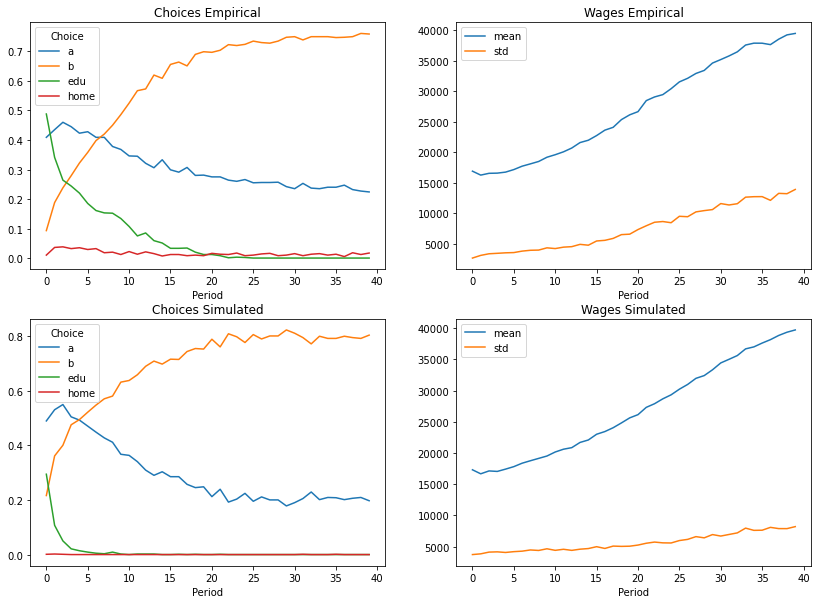
The function defined above will generate the following subplots:

Start value with delta = 0: The moments for the true parameter vector with the exception that delta is set to 0.
Result with delta = 0: The moments for the parameter vector we generate by estimating the misspecified model.
New starting vector correct delta: The moments for the estimated parameter vector with delta set back to its true value, i.e. the starting values for the final estimation.
Final result: The moments for the estimated parameter vector using the starting values generated in the prior step.
Observed: The “true” moments, i.e. the moments generated from the true parameter vector.

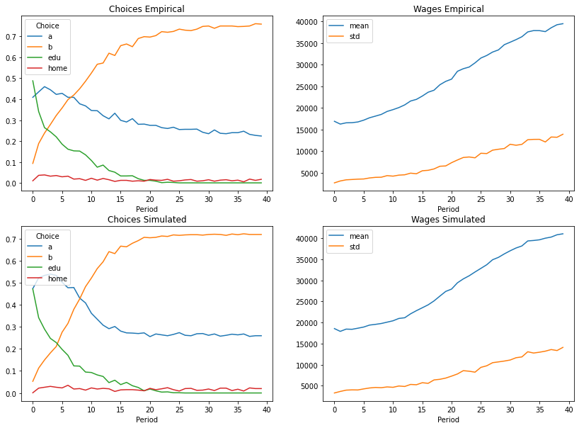
The central plot is (4) Final result since it shows the result at the end of the exercise. We want it to match the “observed” moments as closely as possible. The results overall indicate that the estimation mechanism seems to work, which is what we wanted to test. The criterion function manages to select parameters that improve the match between simulated and observed moments compared to the starting values it is faced with.

The plots also showcase some interesting aspects about the economics of the model. For example, in the first two plots where delta is fixed to zero, no agent chooses education in any period since agents are not forward-looking for this specification.

Choice Frequencies#

[18]:

plot_moments(
    params_dict,
    get_simulated_moments,
    empirical_moments,
    "Choice Frequencies",
    -0.1,
    1.1,
)

../_images/how_to_guides_how_to_msm_estimation_exercise_47_0.png

Wage Distribution#

[19]:

plot_moments(
    params_dict,
    get_simulated_moments,
    empirical_moments,
    "Wage Distribution",
    0,
    80_000,
)

../_images/how_to_guides_how_to_msm_estimation_exercise_49_0.png

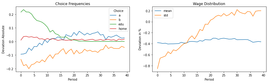
Difference in Moments#

We can also easily compute the difference in moments between the simulated and observed data. For the choices we just look at the total difference in choice frequencies for each period.

[20]:

_, simulated_moments = get_simulated_moments(params_dict["(4) Final result"])

[21]:

diff = {}
diff["Choice Frequencies"] = (
    empirical_moments["Choice Frequencies"] - simulated_moments["Choice Frequencies"]
)

For the wage distribution we compute the relative deviation compared to the values of the empirical moments.

[22]:

diff["Wage Distribution"] = (
    empirical_moments["Wage Distribution"] - simulated_moments["Wage Distribution"]
) / empirical_moments["Wage Distribution"]

Again, we can see that the overall result is close to the observed data. However, for the current estimates the number of individuals choosing education in earlier periods is too low and the number of individuals choosing to work is too high. Furthermore, the mean wage is too high in every period.

[23]:

fig, axes = plt.subplots(1, 2, figsize=(15, 4))
axes = axes.ravel()
for i, (key, label) in enumerate(zip(diff, ["Deviation Absolute", "Deviation in %"])):
    diff[key].plot(title=key, ax=axes[i])
    axes[i].set_ylabel(label)

../_images/how_to_guides_how_to_msm_estimation_exercise_57_0.png

Parameter History#

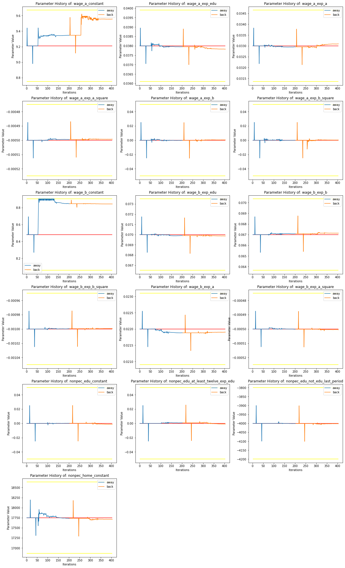
After assessing the criterion value and moment fit of the estimates, we now turn to the parameter values themselves. We can use the parameter history that estimagic saves in the logging databases during optimization to get a picture of how the estimates develop during the exercise and evaluate, which parameters change the most.

[24]:

def plot_params_history(name):
    """ Plot parameter history throughout exercise."""
    values = {}
    for db in ["away", "back"]:
        database = load_database(f"logging_{db}.db")
        params_history = read_last_iterations(
            database, "params_history", 10_000, "pandas"
        )
        values[db] = params_history[name]
        true = params_history.iloc[0]

    values["back"].index = values["back"].index + max(values["away"].index)

    plt.plot(values["away"], label="away")
    plt.plot(values["back"], label="back")
    plt.ylabel("Parameter Value")
    plt.xlabel("Iterations")
    plt.title("Parameter History of: " + name)

    true = values["away"].iloc[0]

    if true == 0:
        lower, upper = -0.05, 0.05
    else:
        lower = true - abs(true * 0.05)
        upper = true + abs(true * 0.05)

    plt.hlines(
        [true, lower, upper],
        min(values["away"].index),
        max(values["back"].index),
        colors=["red", "yellow", "yellow"],
    )
    plt.legend()

The plots below show the parameter history of parameters that affect wages and the non-pecuniary rewards for education and the home option. Shocks and other parameters are purposely left out for legibility. The red line indicates true parameter value and the yellow lines show the bounds set at the beginning of the exercise. The blue lines show the parameter history during optimization of the misspecified model and the orange line shows the second optimization process where we try to retrieve the true values. The plots reveal that most of the pictured parameters did not change much during the whole exercise. The change in moments seems to mainly be driven by the wage constants of the model which increasingly move towards the bounds during the exercise.

Seeing that the wage constants are quite high compared to the true model, it is not surprising that our current specification under-predicts the choice frequencies for the education and home option and over-predicts the choice frequencies of the working alternatives. In the next step we will thus attempt to correct this problem.

[25]:

params_names = params.index.map("_".join)
params_names = params_names[params_names.str.contains("wage|nonpec")]
plt.figure(figsize=(20, 60))
for idx, name in enumerate(params_names):
    plt.subplot(11, 3, idx + 1)
    plot_params_history(name)
    plt.subplots_adjust(top=0.95)

../_images/how_to_guides_how_to_msm_estimation_exercise_61_0.png

Refining Estimation Results#

The results from the exercise lead us to the conclusion that the overall estimation mechanism seem to work well. The optimizer manages to select parameters that improve the match between simulated and empirical moments, even after being led into the wrong direction through a misspecified model. However, our results for the parameter estimates themselves are not satisfactory yet since the model over-predicts the choice frequencies of work options and under-predicts choice frequencies of the other alternatives.

To refine the results, we will thus run an optimization yet again, this time only on the constants of the model. This allows the optimizer to focus only on these four parameters and will prevent it form trying to improve the fit through other parameters like shocks.

For the estimation we use the parameters from step (4) of the exercise as starting values and create new constraints that fix all parameters but the constants.

[26]:

params_start = params_dict["(4) Final result"][["value", "lower", "upper"]]

[27]:

constr = []
constr += [{"loc": "shocks_sdcorr", "type": "sdcorr"}]
# Fix all parameters.
for index in params_start.index:
    constr += [{"loc": index, "type": "fixed"}]
# Free up constants.
for item in constr:
    if "constant" in item["loc"]:
        constr.remove(item)

[28]:

rslt_constants = minimize(
    weighted_sum_squared_errors,
    params=params_start,
    constraints=constr,
    algorithm="nlopt_bobyqa",
    algo_options={"maxeval": 200},
)

The criterion value improves substantially.

[29]:

print("Starting Criterion Value: ", round(weighted_sum_squared_errors(params_start), 1))
print("Result Criterion Value: ", round(weighted_sum_squared_errors(rslt_constants[1]), 1))

Starting Criterion Value:  85052.4
Result Criterion Value:  10110.4

The moment estimates also improve compared to the prior solution.

[30]:

_, simulated_moments = get_simulated_moments(rslt_constants[1])

[31]:

def plot_all_moments(empirical_moments, simulated_moments):
    fig, axes = plt.subplots(nrows=2, ncols=2, figsize=(14, 10))
    empirical_moments["Choice Frequencies"].plot(
        title="Choices Empirical", ax=axes[0, 0]
    )
    empirical_moments["Wage Distribution"].plot(title="Wages Empirical", ax=axes[0, 1])
    simulated_moments["Choice Frequencies"].plot(
        title="Choices Simulated", ax=axes[1, 0]
    )
    simulated_moments["Wage Distribution"].plot(title="Wages Simulated", ax=axes[1, 1])

[32]:

plot_all_moments(empirical_moments, simulated_moments)

../_images/how_to_guides_how_to_msm_estimation_exercise_71_0.png

Finally, after correcting the constants of the model, we can free up the other parameters for estimation one last time.

[33]:

params_start = rslt_constants[1][["value", "lower", "upper"]]

[34]:

constraints = rp.get_parameter_constraints("kw_94_one")
constraints += [{"loc": ("delta", "delta"), "type": "fixed"}]

[35]:

rslt_refined = minimize(
    criterion_msm,
    params=params_start,
    constraints=constraints,
    algorithm="nlopt_bobyqa",
    algo_options={"maxeval": 200},
)

The criterion value improves yet again and the simulated moments seem to match the observed moments fairly well, too. We can still see some discrepancies, especially for the choice frequencies of occupation b which could be removed through further fine-tuning. For the sake of this exercise, we are content with the result.

[36]:

print("Starting Criterion Value: ", round(criterion_msm(params_start), 1))
print("Result Criterion Value: ", round(criterion_msm(rslt_refined[1]), 1))

Starting Criterion Value:  10110.4
Result Criterion Value:  3404.1

[37]:

_, simulated_moments = get_simulated_moments(rslt_refined[1])

[38]:

plot_all_moments(empirical_moments, simulated_moments)

../_images/how_to_guides_how_to_msm_estimation_exercise_79_0.png

References#

Eisenhauer, P., Heckman, J. J., & Mosso, S. (2015). Estimation of dynamic discrete choice models by maximum likelihood and the simulated method of moments. International Economic Review, 56(2), 331-357.

Eisenhauer, P. (2019). The approximate solution of finite‐horizon discrete‐choice dynamic programming models. Journal of Applied Econometrics, 34(1), 149-154.

Keane, M.P. and Wolpin, K.I. (1994). The Solution and Estimation of Discrete Choice Dynamic Programming Models by Simulation and Interpolation: Monte Carlo Evidence. The Review of Economics and Statistics, 76(4): 648-672.

McFadden, D. (1989). A Method of Simulated Moments for Estimation of Discrete Response Models without Numerical Integration. Econometrica: Journal of the Econometric Society, 995-1026.

Additional Resources#

Adda, J., & Cooper, R. W. (2003). Dynamic Economics: Quantitative Methods and Applications. MIT press.

Andrews, I., Gentzkow, M., & Shapiro, J. M. (2017). Measuring the Sensitivity of Parameter Estimates to Estimation Moments. The Quarterly Journal of Economics, 132(4), 1553-1592.

Davidson, R., & MacKinnon, J. G. (2004). Econometric Theory and Methods (Vol. 5). New York: Oxford University Press.

Evans, R. W. (2018, July 5). Simulated Method of Moments (SMM) Estimation. QuantEcon Notes.

Gourieroux, M., & Monfort, D. A. (1996). Simulation-based econometric methods. Oxford university press.

Stern, S. (1997). Simulation-based estimation. Journal of Economic Literature, 35(4), 2006-2039.