View and download the notebook here!
Keane and Wolpin (1994)#
Note that most of the code cells are hidden from this notebook for a better reading flow. Check out the notebook in the documentation folder in the Github repository for more details.
Keane and Wolpin (1994) and the previously published working paper Keane and Wolpin (1994b) generate three different Monte Carlo samples. This notebook replicates some of their results as well as giving other insights into the model.
Some intuitions#
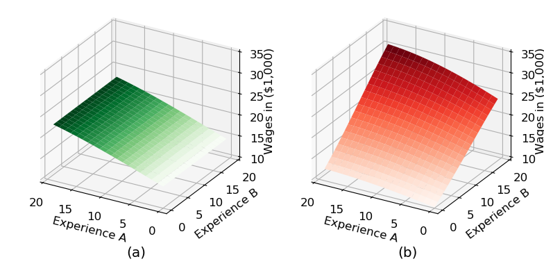
We first plot the returns to experience while holding education constant at the initial ten years. Occupation B is more skill intensive in the sense that own experience has higher return than is the case for Occupation A. There is some general skill learned in Occupation A which is transferable to Occupation B. However, work experience is occupation-specific in Occupation B.
[7]:
fig
[7]:
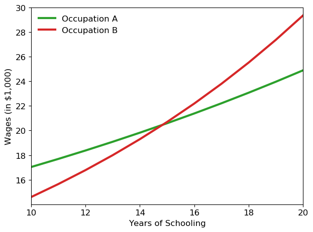
The next figure shows that the returns to schooling are larger in Occupation B. While its initial wage is lower, it does increase faster with schooling compared to Occupation A. The graphs are generated by holding experience in both sectors constant at five years.
[9]:
fig
[9]:
Replication - Effect of college tuition subsidy#
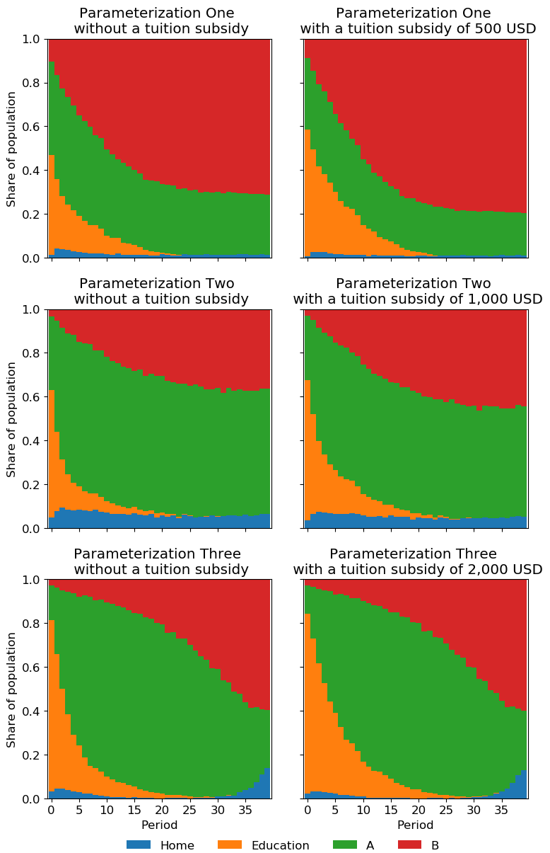
This section replicates Table 6 in Keane and Wolpin (1994) which studies the effect of different amounts of tuition subsidies. First, we are going to show the effect of the tuition subsidy on each of the parametrizations for a sample of 1,000 simulated individuals. After that, Table 6 is replicated where the policy effect is measured as the average difference in experience for 40 samples with 100 invididuals with and without the tutition subsidy. The authors apply a 500 USD tuition subsidy on the first parametrization, 1,000 USD on the second and 2,000 USD on the third parametrization.
The following figures show the impact of the tuition subsidies for each of the parametrizations next to each other.
[12]:
fig
[12]:
The following two tables refer to summary statistics of the tuition subsidy experiment. The first table refers to the replication and the second contains the results from Keane and Wolpin (1994). The tables show the differences in experience between the sample without and with subsidy for all parameterizations. The standard deviations of the mean are computed by simulating 40 bootstrap samples á 100 individuals. All means of the replication lie within one standard deviation.
[14]:
replication
[14]:
| Data Set One | Data Set Two | Data Set Three | |||||||
|---|---|---|---|---|---|---|---|---|---|
| edu | a | b | edu | a | b | edu | a | b | |
| Exact Solution - Mean | 1.449 | -3.450 | 2.213 | 1.116 | -2.685 | 2.004 | 1.693 | -1.349 | -0.212 |
| Exact Solution - Std | 0.217 | 0.987 | 0.887 | 0.236 | 0.622 | 0.516 | 0.226 | 0.242 | 0.111 |
[16]:
table_6
[16]:
| Data Set One | Data Set Two | Data Set Three | |||||||
|---|---|---|---|---|---|---|---|---|---|
| edu | a | b | edu | a | b | edu | a | b | |
| Exact Solution - Mean | 1.44 | -3.43 | 2.19 | 1.12 | -2.71 | 2.08 | 1.67 | -1.27 | -0.236 |
| Exact Solution - Std | 0.18 | 0.94 | 0.89 | 0.22 | 0.53 | 0.43 | 0.20 | 0.18 | 0.100 |
Replication - Choice distributions#
This section replicates the choice distributions for all three parameterizations in Keane and Wolpin (1994b) Table 2.1-2.3. The tables show the share of individuals choosing each choice for each period. The original results are on the left hand side and the replications on the right hand side.
[18]:
table_2_1
[18]:
| Table 2.1 | Replication | |||||||
|---|---|---|---|---|---|---|---|---|
| a | b | edu | home | a | b | edu | home | |
| Period | ||||||||
| 0 | 0.386 | 0.116 | 0.490 | 0.008 | 0.442 | 0.093 | 0.453 | 0.012 |
| 1 | 0.427 | 0.175 | 0.354 | 0.044 | 0.474 | 0.184 | 0.293 | 0.049 |
| 2 | 0.444 | 0.220 | 0.308 | 0.028 | 0.490 | 0.228 | 0.244 | 0.038 |
| 3 | 0.459 | 0.263 | 0.255 | 0.023 | 0.473 | 0.261 | 0.227 | 0.039 |
| 4 | 0.417 | 0.332 | 0.218 | 0.033 | 0.473 | 0.292 | 0.197 | 0.038 |
| 5 | 0.427 | 0.374 | 0.175 | 0.024 | 0.467 | 0.337 | 0.171 | 0.025 |
| 6 | 0.412 | 0.387 | 0.179 | 0.022 | 0.457 | 0.361 | 0.165 | 0.017 |
| 7 | 0.399 | 0.421 | 0.155 | 0.025 | 0.419 | 0.407 | 0.153 | 0.021 |
| 8 | 0.372 | 0.475 | 0.130 | 0.023 | 0.421 | 0.428 | 0.133 | 0.018 |
| 9 | 0.355 | 0.501 | 0.126 | 0.018 | 0.415 | 0.456 | 0.107 | 0.022 |
| 10 | 0.340 | 0.537 | 0.099 | 0.024 | 0.416 | 0.492 | 0.076 | 0.016 |
| 11 | 0.342 | 0.567 | 0.081 | 0.010 | 0.379 | 0.534 | 0.070 | 0.017 |
| 12 | 0.322 | 0.585 | 0.073 | 0.020 | 0.385 | 0.532 | 0.064 | 0.019 |
| 13 | 0.321 | 0.612 | 0.056 | 0.011 | 0.374 | 0.568 | 0.047 | 0.011 |
| 14 | 0.303 | 0.619 | 0.062 | 0.016 | 0.349 | 0.586 | 0.045 | 0.020 |
| 15 | 0.297 | 0.640 | 0.052 | 0.011 | 0.358 | 0.593 | 0.039 | 0.010 |
| 16 | 0.290 | 0.664 | 0.034 | 0.012 | 0.346 | 0.601 | 0.039 | 0.014 |
| 17 | 0.304 | 0.656 | 0.028 | 0.012 | 0.339 | 0.623 | 0.026 | 0.012 |
| 18 | 0.283 | 0.686 | 0.018 | 0.013 | 0.324 | 0.652 | 0.017 | 0.007 |
| 19 | 0.277 | 0.695 | 0.016 | 0.012 | 0.314 | 0.655 | 0.012 | 0.019 |
| 20 | 0.288 | 0.691 | 0.011 | 0.010 | 0.316 | 0.663 | 0.005 | 0.016 |
| 21 | 0.266 | 0.716 | 0.003 | 0.015 | 0.308 | 0.667 | 0.009 | 0.016 |
| 22 | 0.268 | 0.717 | 0.006 | 0.009 | 0.318 | 0.668 | 0.006 | 0.008 |
| 23 | 0.258 | 0.731 | 0.001 | 0.010 | 0.305 | 0.678 | 0.003 | 0.014 |
| 24 | 0.265 | 0.715 | 0.005 | 0.015 | 0.306 | 0.683 | 0.000 | 0.011 |
| 25 | 0.270 | 0.720 | 0.003 | 0.007 | 0.304 | 0.677 | 0.001 | 0.018 |
| 26 | 0.254 | 0.730 | 0.000 | 0.016 | 0.298 | 0.691 | 0.001 | 0.010 |
| 27 | 0.252 | 0.743 | 0.000 | 0.005 | 0.303 | 0.679 | 0.000 | 0.018 |
| 28 | 0.249 | 0.736 | 0.000 | 0.015 | 0.307 | 0.683 | 0.000 | 0.010 |
| 29 | 0.241 | 0.742 | 0.000 | 0.017 | 0.288 | 0.698 | 0.000 | 0.014 |
| 30 | 0.246 | 0.743 | 0.000 | 0.011 | 0.289 | 0.699 | 0.000 | 0.012 |
| 31 | 0.243 | 0.750 | 0.000 | 0.007 | 0.302 | 0.686 | 0.000 | 0.012 |
| 32 | 0.242 | 0.748 | 0.000 | 0.010 | 0.288 | 0.694 | 0.000 | 0.018 |
| 33 | 0.243 | 0.746 | 0.000 | 0.011 | 0.282 | 0.706 | 0.000 | 0.012 |
| 34 | 0.229 | 0.757 | 0.000 | 0.014 | 0.282 | 0.704 | 0.000 | 0.014 |
| 35 | 0.244 | 0.750 | 0.000 | 0.006 | 0.279 | 0.703 | 0.000 | 0.018 |
| 36 | 0.234 | 0.755 | 0.000 | 0.011 | 0.278 | 0.702 | 0.000 | 0.020 |
| 37 | 0.238 | 0.749 | 0.000 | 0.013 | 0.278 | 0.704 | 0.000 | 0.018 |
| 38 | 0.231 | 0.753 | 0.000 | 0.016 | 0.278 | 0.710 | 0.000 | 0.012 |
| 39 | 0.230 | 0.758 | 0.000 | 0.012 | 0.274 | 0.708 | 0.000 | 0.018 |
[20]:
table_2_2
[20]:
| Table 2.2 | Replication | |||||||
|---|---|---|---|---|---|---|---|---|
| a | b | edu | home | a | b | edu | home | |
| Period | ||||||||
| 0 | 0.344 | 0.038 | 0.575 | 0.043 | 0.304 | 0.033 | 0.616 | 0.047 |
| 1 | 0.481 | 0.059 | 0.375 | 0.085 | 0.460 | 0.067 | 0.401 | 0.072 |
| 2 | 0.606 | 0.073 | 0.238 | 0.083 | 0.582 | 0.094 | 0.232 | 0.092 |
| 3 | 0.633 | 0.115 | 0.176 | 0.076 | 0.600 | 0.125 | 0.174 | 0.101 |
| 4 | 0.658 | 0.126 | 0.143 | 0.073 | 0.632 | 0.117 | 0.161 | 0.090 |
| 5 | 0.659 | 0.146 | 0.111 | 0.084 | 0.625 | 0.151 | 0.158 | 0.066 |
| 6 | 0.662 | 0.151 | 0.096 | 0.091 | 0.628 | 0.174 | 0.128 | 0.070 |
| 7 | 0.642 | 0.182 | 0.097 | 0.079 | 0.621 | 0.174 | 0.125 | 0.080 |
| 8 | 0.657 | 0.174 | 0.084 | 0.085 | 0.614 | 0.212 | 0.092 | 0.082 |
| 9 | 0.632 | 0.210 | 0.082 | 0.076 | 0.657 | 0.214 | 0.065 | 0.064 |
| 10 | 0.648 | 0.227 | 0.056 | 0.069 | 0.650 | 0.236 | 0.050 | 0.064 |
| 11 | 0.642 | 0.241 | 0.046 | 0.071 | 0.632 | 0.264 | 0.044 | 0.060 |
| 12 | 0.641 | 0.254 | 0.044 | 0.061 | 0.629 | 0.269 | 0.041 | 0.061 |
| 13 | 0.643 | 0.265 | 0.036 | 0.056 | 0.627 | 0.279 | 0.045 | 0.049 |
| 14 | 0.633 | 0.278 | 0.029 | 0.060 | 0.626 | 0.272 | 0.046 | 0.056 |
| 15 | 0.625 | 0.291 | 0.023 | 0.061 | 0.610 | 0.304 | 0.031 | 0.055 |
| 16 | 0.623 | 0.305 | 0.020 | 0.052 | 0.643 | 0.282 | 0.026 | 0.049 |
| 17 | 0.628 | 0.289 | 0.028 | 0.055 | 0.613 | 0.300 | 0.026 | 0.061 |
| 18 | 0.599 | 0.325 | 0.014 | 0.062 | 0.625 | 0.292 | 0.021 | 0.062 |
| 19 | 0.597 | 0.322 | 0.020 | 0.061 | 0.590 | 0.330 | 0.014 | 0.066 |
| 20 | 0.621 | 0.317 | 0.017 | 0.045 | 0.594 | 0.355 | 0.006 | 0.045 |
| 21 | 0.613 | 0.327 | 0.010 | 0.050 | 0.562 | 0.372 | 0.011 | 0.055 |
| 22 | 0.585 | 0.358 | 0.006 | 0.051 | 0.577 | 0.359 | 0.006 | 0.058 |
| 23 | 0.580 | 0.360 | 0.005 | 0.055 | 0.545 | 0.390 | 0.004 | 0.061 |
| 24 | 0.596 | 0.344 | 0.000 | 0.060 | 0.573 | 0.375 | 0.001 | 0.051 |
| 25 | 0.622 | 0.334 | 0.003 | 0.041 | 0.583 | 0.370 | 0.004 | 0.043 |
| 26 | 0.566 | 0.376 | 0.002 | 0.056 | 0.553 | 0.381 | 0.005 | 0.061 |
| 27 | 0.567 | 0.386 | 0.001 | 0.046 | 0.565 | 0.365 | 0.002 | 0.068 |
| 28 | 0.548 | 0.394 | 0.000 | 0.058 | 0.584 | 0.370 | 0.000 | 0.046 |
| 29 | 0.560 | 0.373 | 0.002 | 0.065 | 0.552 | 0.387 | 0.000 | 0.061 |
| 30 | 0.562 | 0.374 | 0.000 | 0.064 | 0.548 | 0.398 | 0.000 | 0.054 |
| 31 | 0.568 | 0.388 | 0.000 | 0.044 | 0.544 | 0.394 | 0.000 | 0.062 |
| 32 | 0.562 | 0.374 | 0.000 | 0.064 | 0.554 | 0.387 | 0.000 | 0.059 |
| 33 | 0.569 | 0.367 | 0.000 | 0.064 | 0.540 | 0.397 | 0.000 | 0.063 |
| 34 | 0.578 | 0.369 | 0.000 | 0.053 | 0.536 | 0.407 | 0.000 | 0.057 |
| 35 | 0.557 | 0.390 | 0.000 | 0.053 | 0.541 | 0.395 | 0.000 | 0.064 |
| 36 | 0.562 | 0.387 | 0.000 | 0.051 | 0.545 | 0.400 | 0.000 | 0.055 |
| 37 | 0.542 | 0.397 | 0.000 | 0.061 | 0.561 | 0.376 | 0.000 | 0.063 |
| 38 | 0.562 | 0.385 | 0.000 | 0.053 | 0.555 | 0.387 | 0.000 | 0.058 |
| 39 | 0.551 | 0.390 | 0.000 | 0.059 | 0.569 | 0.380 | 0.000 | 0.051 |
[22]:
table_2_3
[22]:
| Table 2.3 | Replication | |||||||
|---|---|---|---|---|---|---|---|---|
| a | b | edu | home | a | b | edu | home | |
| Period | ||||||||
| 0 | 0.169 | 0.036 | 0.752 | 0.043 | 0.153 | 0.028 | 0.769 | 0.050 |
| 1 | 0.308 | 0.042 | 0.594 | 0.056 | 0.315 | 0.048 | 0.585 | 0.052 |
| 2 | 0.455 | 0.058 | 0.430 | 0.057 | 0.463 | 0.054 | 0.418 | 0.065 |
| 3 | 0.574 | 0.066 | 0.326 | 0.034 | 0.544 | 0.067 | 0.321 | 0.068 |
| 4 | 0.628 | 0.070 | 0.255 | 0.047 | 0.631 | 0.064 | 0.258 | 0.047 |
| 5 | 0.710 | 0.071 | 0.189 | 0.030 | 0.682 | 0.076 | 0.200 | 0.042 |
| 6 | 0.725 | 0.080 | 0.166 | 0.029 | 0.741 | 0.076 | 0.156 | 0.027 |
| 7 | 0.746 | 0.090 | 0.139 | 0.025 | 0.760 | 0.077 | 0.124 | 0.039 |
| 8 | 0.752 | 0.090 | 0.132 | 0.026 | 0.758 | 0.103 | 0.111 | 0.028 |
| 9 | 0.762 | 0.101 | 0.123 | 0.014 | 0.795 | 0.103 | 0.081 | 0.021 |
| 10 | 0.782 | 0.115 | 0.083 | 0.020 | 0.816 | 0.107 | 0.063 | 0.014 |
| 11 | 0.797 | 0.120 | 0.071 | 0.012 | 0.788 | 0.129 | 0.069 | 0.014 |
| 12 | 0.793 | 0.129 | 0.070 | 0.008 | 0.799 | 0.127 | 0.065 | 0.009 |
| 13 | 0.782 | 0.153 | 0.059 | 0.006 | 0.808 | 0.123 | 0.056 | 0.013 |
| 14 | 0.788 | 0.148 | 0.055 | 0.009 | 0.801 | 0.144 | 0.047 | 0.008 |
| 15 | 0.779 | 0.158 | 0.054 | 0.009 | 0.787 | 0.162 | 0.045 | 0.006 |
| 16 | 0.783 | 0.173 | 0.042 | 0.002 | 0.790 | 0.167 | 0.035 | 0.008 |
| 17 | 0.775 | 0.182 | 0.035 | 0.008 | 0.771 | 0.183 | 0.037 | 0.009 |
| 18 | 0.776 | 0.192 | 0.029 | 0.003 | 0.773 | 0.183 | 0.037 | 0.007 |
| 19 | 0.763 | 0.208 | 0.028 | 0.001 | 0.757 | 0.208 | 0.028 | 0.007 |
| 20 | 0.757 | 0.218 | 0.022 | 0.003 | 0.754 | 0.224 | 0.019 | 0.003 |
| 21 | 0.740 | 0.235 | 0.020 | 0.005 | 0.735 | 0.246 | 0.015 | 0.004 |
| 22 | 0.704 | 0.280 | 0.014 | 0.002 | 0.709 | 0.278 | 0.010 | 0.003 |
| 23 | 0.712 | 0.274 | 0.012 | 0.002 | 0.708 | 0.280 | 0.009 | 0.003 |
| 24 | 0.712 | 0.269 | 0.013 | 0.006 | 0.703 | 0.282 | 0.010 | 0.005 |
| 25 | 0.698 | 0.290 | 0.008 | 0.004 | 0.645 | 0.335 | 0.011 | 0.009 |
| 26 | 0.657 | 0.332 | 0.004 | 0.007 | 0.646 | 0.342 | 0.008 | 0.004 |
| 27 | 0.625 | 0.368 | 0.003 | 0.004 | 0.630 | 0.357 | 0.006 | 0.007 |
| 28 | 0.628 | 0.369 | 0.001 | 0.002 | 0.617 | 0.376 | 0.002 | 0.005 |
| 29 | 0.587 | 0.396 | 0.004 | 0.013 | 0.595 | 0.395 | 0.003 | 0.007 |
| 30 | 0.557 | 0.433 | 0.001 | 0.009 | 0.549 | 0.430 | 0.001 | 0.020 |
| 31 | 0.541 | 0.452 | 0.000 | 0.007 | 0.525 | 0.454 | 0.002 | 0.019 |
| 32 | 0.516 | 0.468 | 0.000 | 0.016 | 0.512 | 0.467 | 0.002 | 0.019 |
| 33 | 0.494 | 0.484 | 0.001 | 0.021 | 0.456 | 0.512 | 0.000 | 0.032 |
| 34 | 0.445 | 0.518 | 0.000 | 0.037 | 0.425 | 0.533 | 0.000 | 0.042 |
| 35 | 0.388 | 0.571 | 0.000 | 0.041 | 0.393 | 0.557 | 0.000 | 0.050 |
| 36 | 0.370 | 0.575 | 0.001 | 0.054 | 0.350 | 0.579 | 0.000 | 0.071 |
| 37 | 0.329 | 0.584 | 0.000 | 0.087 | 0.345 | 0.560 | 0.000 | 0.095 |
| 38 | 0.306 | 0.595 | 0.000 | 0.099 | 0.304 | 0.592 | 0.000 | 0.104 |
| 39 | 0.270 | 0.604 | 0.000 | 0.126 | 0.283 | 0.569 | 0.000 | 0.148 |
References#
Keane, M. P. and Wolpin, K. I. (1994). The Solution and Estimation of Discrete Choice Dynamic Programming Models by Simulation and Interpolation: Monte Carlo Evidence. The Review of Economics and Statistics, 76(4): 648-672.
Keane, M. P. and Wolpin, K. I. (1994b). The Solution and Estimation of Discrete Choice Dynamic Programming Models by Simulation and Interpolation: Monte Carlo Evidence. Federal Reserve Bank of Minneapolis, No. 181.