The Economic Model¶

Introduction¶

Keane and Wolpin (1997) develop a model in which an agent decides among \(M\) possible alternatives in each of \(T\) (finite) discrete periods of time. Alternatives are defined to be mutually exclusive and \(d_m(a) = 1\) indicates that alternative \(m\) is chosen at time (age) \(a\) and \(d_m(a) = 0\) indicates otherwise. Associated with each choice is an immediate reward \(R_m(S(a))\) that is known to the agent at time \(a\) but partly unknown from the perspective of periods prior to \(a\). All the information known to the agent at time \(a\) that affects immediate and future rewards is contained in the state space \(S(a)\).

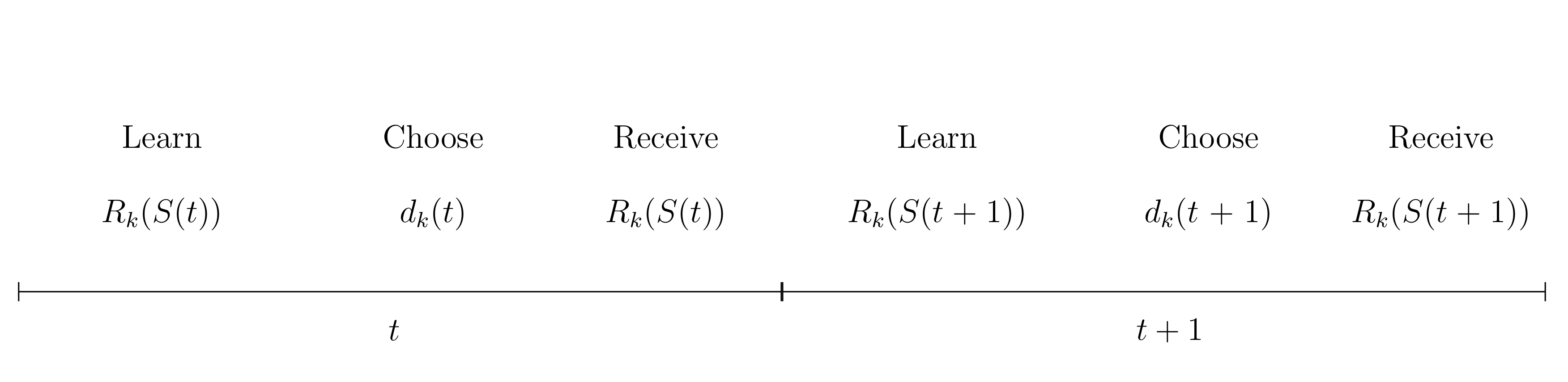
We depict the timing of events below. At the beginning of period \(a\) the agent fully learns about all immediate rewards, chooses one of the alternatives and receives the corresponding benefits. The state space is then updated according to the agent’s state experience and the process is repeated in \(a + 1\).

Agents are forward looking. Thus, they do not simply choose the alternative with the highest immediate rewards each period. Instead, their objective at any time \(\tau\) is to maximize the expected rewards over the remaining time horizon:

\[\max_{\{d_m(a)\}_{m \in M}} E\left[ \sum_{\tau = a}^T \delta^{\tau - a} \sum_{m\in M}R_m(\tau)d_m(\tau)\Bigg| S(a)\right]\]

The discount factor \(0 > \delta > 1\) captures the agent’s preference for immediate over future rewards. Agents maximize the equation above by choosing the optimal sequence of alternatives \(\{d_m(a)\}_{m \in M}\) for \(a = \tau, .., T\).

Within this more general framework, Keane and Wolpin (1997) consider the case where agents are risk neutral and each period choose one of five sectors:

work in occupation A (in the paper: white-collar)
work in occupation B (in the paper: blue-collar)
work in occupation C (in the paper: the military)
continue education
remain at home

Details of the Notation¶

In addition, individuals belong to one of K types that determine their base skill / preference endowments in each of the sectors.

Meaning of Subscripts

Notation	Interpretation	Additional Information
m	sectors	1: white-collar, 2: blue-collar, 3: military, 4: school, 5: home
k	endowment type	k = 1, 2, 3, 4 in the extended KW model
a	age /period from \(a_0\) to A	from 16 to 65 in the extended KW model

Each of the five sectors is associated with a reward. The rewards depend on the individual’s base endowments and its experience in the different sectors, its age and schooling level which together determine the individual’s skill in each of the five sectors.

State-Space Variables

Notation	Interpretation	Additional Information
\(S_{a_0}\)	state space at model start	\(S(16)\) in the paper, contains the type of the individual
a	age	from 16 to 65 in the extended KW model
g	schooling	years of schooling
x	work experience	vector: one value for white-collar, blue-collar and military
\(d_1(a-1)\)	whether occ. A was chosen last period
\(d_2(a-1)\)	whether occ. B was chosen last period
\(d_4(a-1)\)	whether education was chosen last period

Other Notation

Notation	Interpretation	Additional Information
\(d_m(a)\)	dummy if sector m was chosen at age a
\(1[]\)	indicator function	1 if statement in [] is true, 0 else

The Reward Functions and Their Parameters¶

In what follows, we take a detailed look at the rewards of each alternative individuals can choose. Some of the rewards of finishing high school and college are universal to all sectors (\(\beta_1 1[g(a) \geq 12] + \beta_2 1[g(a) \geq 16]\)).

In contrast to Keane & Wolpin (1997) here all linear indices only carry positive signs as this is how parameters are specified in the model specification.

Occupation A¶

The instantaneous reward associated with working in occupation A is given by the following equation:

\[\begin{split}R_{1,k}(a) = r_1 \cdot e_{1,k}(a) &+ c_{1,1} \cdot 1[d_1(a-1) = 0] + c_{1,2} \cdot 1[x_1(a) = 0]\\ &+ \alpha_1 + \beta_1 \cdot 1[g(a) \geq 12]\\ &+ \beta_2 \cdot 1[g(a) \geq 16] + \beta_3 \cdot 1[x_3(a) = 1],\end{split}\]

where \(e_{1,k}(a)\) are the current skills of an individual of type \(k\) in white-collar work. They evolve according to the following law:

\[\begin{split}e_{1,k}(a) = \exp\{\\ e_{1,k}(a_0) &+ e_{1,11} \cdot g(a) + e_{1,12} \cdot 1[g(a) \geq 12]\\ &+ e_{1,13} \cdot 1[g(a) \geq 16] + e_{1,2} \cdot x_1(a)\\ &+ e_{1, 3} \cdot x^2_1(a) + e_{1,4} \cdot 1[x_1 > 0)]\\ &+ e_{1, 5} \cdot a + e_{1, 6} \cdot 1[a < 18]\\ &+ e_{1, 7} \cdot d_1(a-1) + e_{1,8} \cdot x_{2}(a)\\ &+ e_{1, 9} \cdot x_3(a)\\ \} \cdot \exp[\epsilon_1(a)],\end{split}\]

where \(\epsilon_1(a)\) is the idiosyncratic, serially uncorrelated shock to the individual’s skills in age a. Note that in Appendix C of Keane & Wolpin (1997) the age function is not necessarily linear (\(e_{1, 5}(a)\)). However, from table 7 it becomes clear that the age function was estimated to be linear so this is what is also implemented in respy.

Furthermore, Keane & Wolpin (1997) only allow for a second degree polynomial function for the same sector experience. Respy allows for both civilian sectors (occupation A and B) to have quadratic effects on wages in both sectors.

Notation	Interpretation
.	coefficients of the skill technology function
\(ln(r_1)\)	skill rental price if the base skill endowment of type 1 (e_{11}(16)) is normalized to 0.
\(e_{1,11}\)	linear return to an additional year of schooling
\(e_{1,2}\)	return to experience, same sector, linear
\(e_{1,3}\)	return to experience, same sector, quadratic (divided by 100)
\(e_{1,8}\)	return to experience, other civilian sector, linear
not present in KW 97	return to experience, other civilian sector, quadratic (divided by 100)
\(e_{1,12}\)	skill premium of having finished high school
\(e_{1,13}\)	skill premium of having finished college
\(e_{1,5}\)	linear age effect
\(e_{1,6}\)	effect of being a minor
\(e_{1,4}\)	gain from having worked in the occupation at least once before
\(e_{1,7}\)	gain from remaining in the same occupation as in previous period
.	other coefficients of the reward function
\(\alpha_1\)	constant
\(c_{1,1}\)	reward of switching to A from other occupation
\(c_{1,2}\)	reward of working in A for the first time

Occupation B¶

The instantaneous reward associated with working in occupation B is analogous to that of occupation A and given by the following function:

\[\begin{split}R_{2,k}(a) = r_2 \cdot e_{2,k}(a) &+ c_{2,1} \cdot 1[d_1(a-1) = 0] + c_{2,2} \cdot 1[x_2(a) = 0]\\ &+ \alpha_2 + \beta_1 \cdot 1[g(a) \geq 12]\\ &+ \beta_2 \cdot 1[g(a) \geq 16] + \beta_3 \cdot 1[x_3(a) = 1],\end{split}\]

where \(e_{2,k}(a)\) are the current skills of the individual in blue-collar work. They evolve according to the following law:

\[\begin{split}e_{2,k}(a) = \exp\{\\ e_{2,k}(a_0) &+ e_{2,11} \cdot g(a) + e_{2,12} \cdot 1[g(a) \geq 12]\\ &+ e_{2,13} \cdot 1[g(a) \geq 16] + e_{2,2} \cdot x_2(a)\\ &+ e_{2, 3} \cdot x^2_2(a) + e_{2,4} \cdot 1[x_2 > 0)]\\ &+ e_{2, 5} \cdot a + e_{2, 6} \cdot 1[a < 18]\\ &+ e_{2, 7} \cdot d_1(a-1) + e_{2,8} \cdot x_{1}(a)\\ &+ e_{2, 9} \cdot x_3(a)\\ \} \cdot \exp[\epsilon_2(a)]\end{split}\]

The same comments as for occupation A apply.

Notation	Interpretation
.	coefficients of the skill technology function
\(ln(r_2)\)	skill rental price if the base skill endowment of type 1 (e_{21}(16)) is normalized to 0.
\(e_{2,11}\)	linear return to an additional year of schooling
\(e_{2,8}\)	return to experience, other civilian sector, linear
not present in KW 97	return to experience, other civilian sector, quadratic, (divided by 100)
\(e_{2,2}\)	return to experience, same sector, linear
\(e_{2,3}\)	return to experience, same sector, quadratic, (divided by 100)
\(e_{2,12}\)	skill premium of having finished high school
\(e_{2,13}\)	skill premium of having finished college
\(e_{2,5}\)	linear age effect
\(e_{2,6}\)	effect of being a minor
\(e_{2,4}\)	gain from having worked in the occupation at least once before
\(e_{2,7}\)	gain from remaining in the same occupation as in previous period
.	other coefficients of the reward function
\(\alpha_2\)	constant
\(c_{2,1}\)	reward of switching to B from other occupation
\(c_{2,2}\)	reward of working in B for the first time

Occupation C¶

The instantaneous reward associated with working in occupation C is different from occupation A and B in several aspects:

In the skill technology function:
- all types have the same base skill endowment in the military (can be seen in table 7, although the state space on page 521 suggests something different).
- no sheep skin effects for finishing high school or college (\(e_{m,12}, e_{m,13}\))
- no effects of civilian sector experiences on the military skills
- no effect of switching to the military from another sector (\(e_{m, 7}\))
In the general reward function:
- The non-pecuniary reward (\(\alpha\)) is multiplicative and not additive (see note below on how it is nevertheless identified)
- The non-pecuniary reward (\(\alpha\)) varies with age (but skills are not allowed to change with age)
- no penalty of leaving the military prematurely (\(\beta_3 \cdot 1[x_3(a) = 1]\))
- There is no reward or penalty for never having worked in the military before (\(1[d_3(a-1) = 0]\))

The reward function is given by the following equation:

\[\begin{split}R_{3,k}(a) = \exp[\alpha_3(a)] \cdot r_3 \cdot e_3(a) + c_{3,2} \cdot 1[x_3(a) = 0] + \\ & \beta_1 \cdot 1[g(a) \geq 12] + \beta_2 \cdot 1[g(a) \geq 16] \cdot exp\{\epsilon_3(a)\}\end{split}\]

where \(e_{3}(a)\) are the current skills of the individual in military work. They evolve according to the following law:

\[\begin{split}e_{3}(a) = exp \{ & e_3(a_0) + e_{3,1} \cdot g(a) + e_{3,2} \cdot x_3(a) + e_{3,3} \cdot x_3^2(a) + \\ & e_{3,4} \cdot 1[x_3 > 0] + e_{3,5}(a) + e_{3, 6} \cdot 1[a < 18]\}\end{split}\]

Notation	Interpretation
.	coefficients of the skill technology function

\(ln(r_3) + e_3(16)\)	skill rental price if the base skill endowment is normalized to 0. (all types start with the same military skill endowment)
\(e_{31}\)	linear return to an additional year of schooling
\(e_{32}\)	return to experience, same sector, linear
\(e_{33}\)	return to experience, same sector, quadratic (divided by 100)
\(e_{34}\)	gain from having worked in the occupation at least once before
\(e_{35}\)	linear age effect
\(e_{36}\)	effect of being a minor
.	other coefficients of the reward function
\(\alpha_{3,c}\)	constant in the non-pecuniary reward
\(\alpha_{3, l}\)	linear age trend in the non-pecuniary reward
\(c_{32}\)	non-pecuniary reward of working in the military for the first time
\(\tilde{\beta}_3\)	benefit of not leaving the military prematurely

Note that the coefficients of the skill technology function are identified by the wage data separately from the other coefficients. Thus, both a constant factor (\(r_3 \cdot exp(e_3(a_0))\)) in the wage part and a constant factor (\(\alpha_{3,c}\)) in the non-pecuniary part can be identified. However, \(r_3 \cdot exp(e_3(a_0))\) can only be estimated jointly.

Note

In the text of the paper it appears that there is a cost of leaving the military sector prematurely that is effective in all sectors but the military (\(\beta_3\). The result table (Table 7), however, suggests that a similar channel was captured by a benefit of not leaving the military sector prematurely that is only effective in the military sector. We implement this second version.

Furthermore, from table 7 it becomes again apparent that the unspecified functions \(\alpha (a)\) and \(e_{3,5}(a)\) are linear in age and \(exp\{\epsilon_3(a)\}\) is missing in the formulas of Appendix C but mentioned in the text.

Schooling¶

The instantaneous utility of schooling is:

\[\begin{split}R_{4,k}(a) = & e_{4,k}(a_0) + tc_1 \cdot 1[g(a) \geq 12] + tc_2 \cdot 1[g(a) \geq 16] + \\ & rc_1 \cdot 1[d_4(a-1) = 0, g(a) < 12] + \\ & rc_2 \cdot 1[d_4(a-1) = 0, g(a) \geq 12] + \\ & \beta_1 \cdot 1[g(a) \geq 12] + \beta_2 \cdot 1[g(a) \geq 16] + \\ & \beta_3 \cdot 1[x_3(a) = 1] + \gamma_{4,1} \cdot a + \\ & \gamma_{4,2} \cdot 1[a < 18]+ \epsilon_4(a)\end{split}\]

Education Sector Parameters

Notation	Interpretation
\(e_{41}(16)\)	constant, consumption value of school attendance for type 1
\(tc_1\)	consumption value of college
\(tc_2\)	consumption value of graduate school
\(rc_2\)	reward for going back to college
\(rc_1\)	reward for of going back to high school
\(\gamma_{41}\)	linear effect of age
\(\gamma_{42}\)	effect of being a minor

There are no skills in education that evolve over time. However, each type has a different base endowment \(e_{4, k}(a_0)\) that affects how much utility this type derives from going to school.

Home Sector¶

The instantaneous utility of staying home is:

\[\begin{split}R_{5,k}(a) = & e_{5,k}(a_0) + \beta_1 \cdot 1[g(a) \geq 12] + \beta_2 \cdot 1[g(a) \geq 16] + \\ & \beta_3 \cdot 1[x_3(a) = 1] + \gamma_{5, 1} \cdot 1[18 \leq a \leq 20] + \gamma_{5, 2} 1[a \geq 21] + \epsilon_5(a)\end{split}\]

Home Sector Parameters

Notation	Interpretation
\(e_{51}(16)\)	mean value of non-market alternative of type 1
\(\gamma_{51}\)	additional value of staying home if aged 18-20
\(\gamma_{52}\)	additional value of staying home if 21 or older

There are no skills in home production that evolve over time. However, each type has a different base endowment \(e_{5, k}(a_0)\) that affects how much utility this type derives from staying home.

The Role of Shocks in the Model¶

The \(\epsilon_{m}(a)\) are alternative-specific shocks to occupational productivity, to the consumption value of schooling, and to the value of non-market time. The productivity and taste shocks follow a five-dimensional multivariate normal distribution with mean zero and covariance matrix \(\Sigma = [\sigma_{m, m'}]\). The realizations are independent across time.

Given the structure of the reward functions and the agent’s objective, the state space at time \(a\) is:

\[\begin{split}S(a) = \{& S(a_0), a, g(a), x_{1}(a), x_{2}(a), x_{3}(a), \\ & d_1(a - 1), d_2(a - 1), d_4(a - 1),\\ & \epsilon_{1}(a), \epsilon_{2}(a),\epsilon_{3}(a),\epsilon_{4}(a), \epsilon_{5}(a)\}.\end{split}\]

It is convenient to denote its observable elements as \(\bar{S}(a)\). The elements of \(S(a)\) evolve according to:

\[ \begin{align}\begin{aligned}x_{1}(a+1) &= x_{1}(a) + d_1(a)\\x_{2}(a+1) &= x_{2}(a) + d_2(a)\\x_{3}(a+1) &= x_{3}(a) + d_3(a)\\g(a+1) &= g(a) + d_4(a)\\f(\epsilon_{t+1}\mid S(t), d_k(t)) &= f(\epsilon_{t+1}\mid \bar{S}(t), d_k(t)), \forall k \in \{1, 2, 3, 4, 5\}\end{aligned}\end{align} \]

where the last equation reflects the fact that the \(\epsilon_{k, t}\)’s are serially independent. We set \(x_{1}(a_0) = x_{2}(a_0) = x_{3}(a_0) = 0\) as the initial conditions.